Lecture 18: Linear Mixed Models and Generalized Linear Mixed Models

1 Learning Objectives

By the end of this lecture, students will be able to:

Extend hierarchical normal models to hierarchical regression settings
Derive full conditional distributions for Gibbs sampling in LME models
Implement Metropolis-Hastings algorithms for GLMMs
Apply hierarchical Poisson regression to real-world count data

2 Linear Mixed Effects Model/Hierarchical regression

\[ Y_{i, j}=\underline{\beta}_{j}^{T} \underline{x}_{i, j}+\varepsilon_{i, j},\qquad \varepsilon_{i, j} \sim \text { i.i.d. }N\left(0, \sigma^{2}\right) \text {, } \]

Data

\(Y_{i, j}\) = math score for student \(i\) in school \(j\)
\(\underline{x}_{i, j}\) = covariate vector for student \(i\) in school \(j\) (intercept and SES)
\(i \in\{1, \ldots, n_{j}\}\) index of students within school \(j\).
\(j \in\{1, \ldots, m\}\) index of schools.

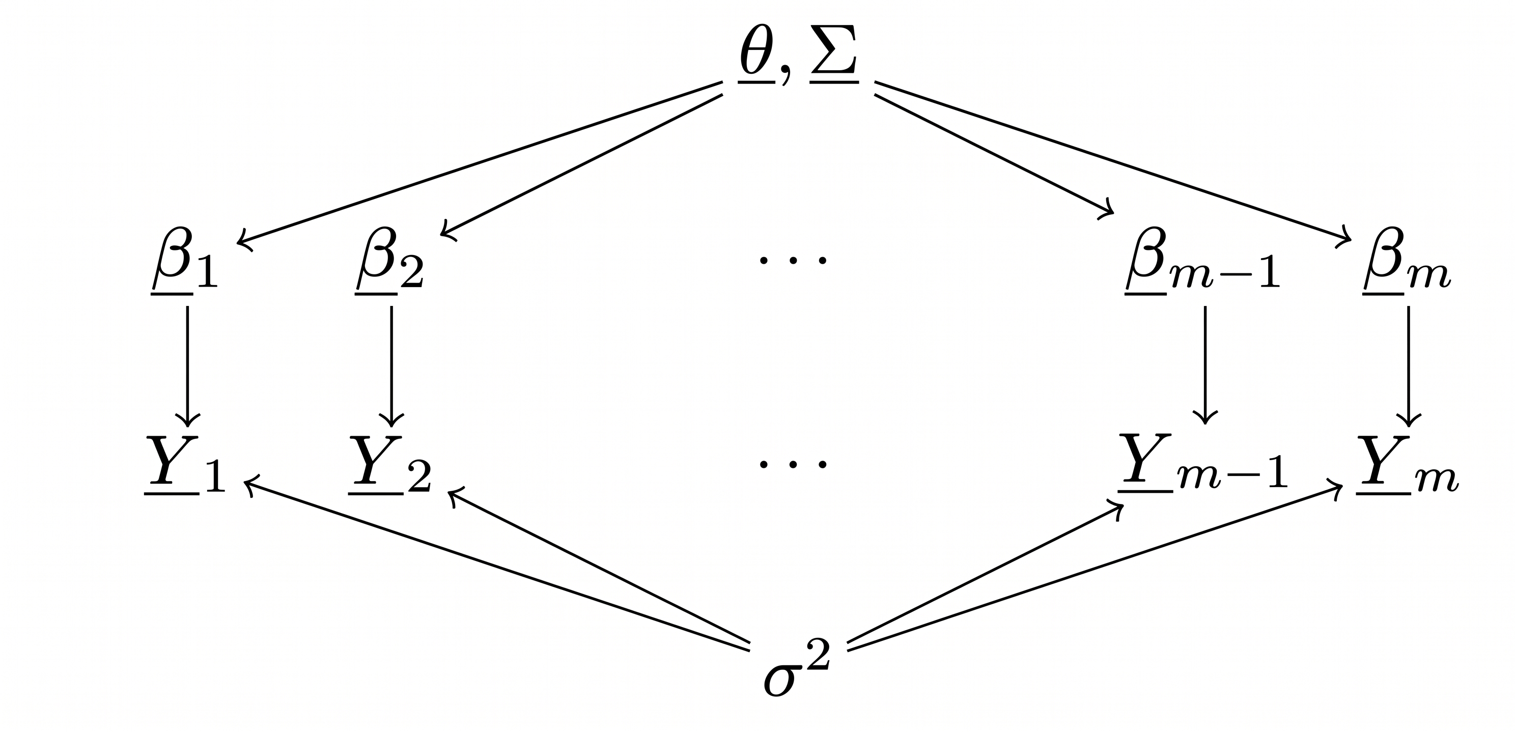
A graphical representation of the hierarchical normal regression model.

DAG for the hierarchical regression model

Figure 1: Bayesian network for the hierarchical regression model

Where we have seen such derivations before?

\[ \begin{aligned} \underline{\beta}_{j} &\mid \underline{y}_{j}, \underline{X}_{j}, \underline{\theta}, \underline{\Sigma}, \sigma^{2} &\\ &&\\ \underline{\theta} &\mid \underline{y}_{j}, \underline{X}_{j}, \underline{\beta}_j, \underline\Sigma, \sigma^{2} &\\ &&\\ \underline{\Sigma} &\mid \underline{y}_{j}, \underline{X}_{j}, \underline{\theta}, \underline{\beta}_j, \sigma^{2} &\\ &&\\ \underline{\sigma}^2 &\mid \underline{y}_{j}, \underline{X}_{j}, \underline{\theta}, \underline\Sigma, \underline{\beta}_j &\\ \end{aligned} \]

3 Full conditional Distributions

Priors

\[ \begin{aligned} \underline{\theta} & \sim \operatorname{MVN} \left(\underline{\mu}_{0}, \Lambda_{0}\right) \\ \underline{\Sigma} & \sim \operatorname{Inverse-Wishart}\left(\eta_{0}, \underline{S}_{0}^{-1}\right) \\ \sigma^{2} & \sim \operatorname{Inverse-Gamma}\left(\nu_{0} / 2, \nu_{0} \sigma_{0}^{2} / 2\right) \end{aligned} \]

Sampling Model

\[ \underline{\beta}_{1}, \ldots, \underline{\beta}_{m} \sim \text { i.i.d. } \text{MVN}(\underline{\theta}, \Sigma) \]

Full conditional Distributions for \(\underline{\beta}_1,\ldots,\underline{\beta}_m\)

\[ \begin{aligned} \underline{\beta}_{j} \mid \underline{y}_{j}, \underline{X}_{j}, \underline{\theta}, \underline\Sigma, \sigma^{2} &\sim {MVN}(m_j,V_j)\\ V_j&=\operatorname{Var}\left[\underline{\beta}_{j} \mid \underline{y}_{j}, \underline{X}_{j}, \sigma^{2}, \underline{\theta}, \underline\Sigma\right] =\left(\Sigma^{-1}+\underline{X}_{j}^{T} \underline{X}_{j} / \sigma^{2}\right)^{-1} \\ m_j&=\mathrm{E}\left[\underline{\beta}_{j} \mid \underline{y}_{j}, \underline{X}_{j}, \sigma^{2}, \underline{\theta}, \underline\Sigma\right] =\left(\underline\Sigma^{-1}+\underline{X}_{j}^{T} \underline{X}_{j} / \sigma^{2}\right)^{-1}\left(\underline\Sigma^{-1} \underline{\theta}+\underline{X}_{j}^{T} \underline{y}_{j} / \sigma^{2}\right) \end{aligned} \]

Full conditional Distributions for \(\underline\theta,\underline\Sigma\)

\[ \begin{aligned} \underline{\theta} \mid \underline{\beta}_{1}, \ldots, \underline{\beta}_{m}, \Sigma & \sim \text { MVN}\left(\underline{\mu}_{m}, \underline\Lambda_{m}\right), \text { where } \\ \underline\Lambda_{m} & =\left(\underline\Lambda_{0}^{-1}+m \underline\Sigma^{-1}\right)^{-1} \\ \underline{\mu}_{m} & =\underline\Lambda_{m}\left(\underline\Lambda_{0}^{-1} \underline{\mu}_{0}+m \underline\Sigma^{-1} \overline{\underline{\beta}}\right) \end{aligned} \]

\[ \begin{aligned} \underline\Sigma \mid \underline{\theta}, \underline{\beta}_{1}, \ldots, \underline{\beta}_{m} & \sim \text { Inverse-Wishart}\left(\eta_{0}+m,\left[\underline{S}_{0}+\underline{S}_{\theta}\right]^{-1}\right), \text { where } \\ \underline{S}_{\theta} & =\sum_{j=1}^{m}\left(\underline{\beta}_{j}-\underline{\theta}\right)\left(\underline{\beta}_{j}-\underline{\theta}\right)^{T} . \end{aligned} \]

Full conditional Distributions for \(\sigma^2\)

\[ \begin{aligned} \sigma^{2}\mid\underline{y},\underline{X},\underline{\beta}_1,\ldots,\underline{\beta}_m & \sim \text {IG}\left(\left[\nu_{0}+\sum n_{j}\right] / 2,\left[\nu_{0} \sigma_{0}^{2}+\mathrm{SSR}\right] / 2\right), \text { where } \\ \mathrm{SSR} & =\sum_{j=1}^{m} \sum_{i=1}^{n_{j}}\left(y_{i, j}-\underline{\beta}_{j}^{T} \underline{x}_{i, j}\right)^{2} . \end{aligned} \]

Results: WWaBD

Posterior estimates of school-specific regression lines (gray) with population mean (black).

Effective Sample Sizes for MCMC Parameters
\[\sigma^2\]	\[\theta_1\]	\[\theta_2\]	\[\Sigma_{11}\]	\[\Sigma_{21}\]	\[\Sigma_{12}\]	\[\Sigma_{22}\]
849	1000	1000	1000	1000	1000	668

For the parameters \(\beta_{0,j}\) and \(\beta_{1,j}\) the easiest way to assess the quality of the MCMC chain is to look at the plot of the posterior mean of \(\beta_{0,j}\) and \(\beta_{1,j}\) versus their ESS for all schools.

Q: Do you see shrinkage? Which schools are shrunk more?

4 Generalized Linear Mixed Effects Model/Hierarchical GLM

In the previous section, we assumed normally distributed responses. But what if our data are counts, binary outcomes, or other non-normal types? We now extend our framework to handle these cases.

Hierarchical LM. Hierarchical GLM.

Within Sampling Model

\[ \begin{aligned} p(\underline{y}_{j} \mid \underline{X}_{j}, \underline{\beta}_{j}) & =\hspace{10cm}\\ \end{aligned} \]

5 Metropolis-Hastings=Metropolis+Gibbs

5.1 Gibbs steps for \((\underline{\theta},\underline{\Sigma})\)

\[ \\[3cm] \]

5.2 Metropolis step for \(\underline{\beta}_j\)

Sample \(\underline{\beta}_{j}^{*} \sim\) multivariate normal \(\left(\underline{\beta}_{j}^{(s)}, V_{j}^{(s)}\right)\).
Compute the acceptance ratio

\[ r=\frac{p\left(\underline{y}_{j} \mid \underline{X}_{j}, \underline{\beta}_{j}^{*}\right) p\left(\underline{\beta}_{j}^{*} \mid \underline{\theta}^{(s)}, \underline\Sigma^{(s)}\right)}{p\left(\underline{y}_{j} \mid \underline{X}_{j}, \underline{\beta}_{j}^{(s)}\right) p\left(\underline{\beta}_{j}^{(s)} \mid \underline{\theta}^{(s)}, \underline\Sigma^{(s)}\right)} \]

Sample \(u \sim\) uniform \((0,1)\). Set \(\underline{\beta}_{j}^{(s+1)}\) to \(\underline{\beta}_{j}^{*}\) if \(u<r\) and to \(\underline{\beta}_{j}^{(s)}\) if \(u>r\).

5.3 A Metropolis-Hastings approximation algorithm

Given current values at scan \(s\) of the Markov chain, we obtain new values as follows:

Sample \(\underline{\theta}^{(s+1)}\) from its full conditional distribution.
Sample \(\underline\Sigma^{(s+1)}\) from its full conditional distribution.
For each \(j \in\{1, \ldots, m\}\),

propose a new value \(\underline{\beta}_{j}^{*}\);
set \(\underline{\beta}_{j}^{(s+1)}\) equal to \(\underline{\beta}_{j}^{*}\) or \(\underline{\beta}_{j}^{(s)}\) with the appropriate probability.

\[ \\[5cm] \]

6 Dataset: Tumor location data

Context: Spatial distribution of tumors in mice along a one-dimensional axis.

6.1 Dataset:

#### Tumor location example
load("../data/tumorLocation.RData") 
Y<-tumorLocation 
t(head(Y,13))

      [,1] [,2] [,3] [,4] [,5] [,6] [,7] [,8] [,9] [,10] [,11] [,12] [,13]
loc1     1    0    1    1    1    0    0    1    3     0     0     0     0
loc2     0    1    0    2    1    0    0    1    0     0     0     0     0
loc3     0    0    0    0    0    0    2    0    2     1     1     0     1
loc4     0    1    0    0    2    0    0    1    2     1     0     0     0
loc5     0    0    1    0    3    0    0    0    1     0     1     2     1
loc6     0    3    1    2    2    2    0    0    0     0     1     0     2
loc7     1    1    0    0    1    3    1    1    0     0     0     1     1
loc8     1    2    0    0    2    0    0    2    0     1     0     2     2
loc9     1    4    1    2    2    0    0    0    1     2     3     4     2
loc10    3    0    2    1    5    1    2    4    4     1     3     3     3
loc11    3    3    2    4    6    2    2    4    5     3     3     3     8
loc12    3    5    3    2    6    3    6    8    7     5     4     3     4
loc13    7    3    5    8    6    7   12    7    9    11    10     8     9
loc14    8    4    5    5    7   10    5    9    9     9     9     6    13
loc15    8    7   10    4    6   12    9   11    6     7     9     7     9
loc16   11    6   10    8    9   10    5   12    9    13    13     8    11
loc17    2    4    8    9    8    9    8    9   13     5     8    13    16
loc18    3    2    9    7    8    9    6    9    6     2     4     3     2
loc19    2    2    3    2    2    4    6    3    2     1     2     1     1
loc20    1    2    0    1    3    0    1    2    2     0     0     0     0

Variables: - \(Y_{j,x}\) = number of tumors at location \(x\) for mouse \(j\) - \(x \in \{0.05, 0.10, \ldots, 0.95, 1.00\}\) (20 locations) - \(j \in \{1, 2, \ldots, 21\}\) (21 mice)

Model: Hierarchical Poisson regression \[ Y_{j,x} \sim \text{Poisson}(\exp(\underline{\beta}_j^T \underline{x})) \] where \(\underline{x}\) includes polynomial basis functions of location.

\[ \\[10cm] \]

EDA: Exploratory data analysis

\[ \\[6cm] \]

Choosing predictors for the hierarchical Poisson regression

7 Results of the Tumor Location dataset analysis

#### MCMC with Caching
cache_file <- "../cache/lecture18_cache.RData"
if(!dir.exists("../cache")) dir.create("../cache", recursive = TRUE)

rmvnorm <- function(n, mu, Sigma) { 
    E <- matrix(rnorm(n * length(mu)), n, length(mu))
    t(t(E %*% chol(Sigma)) + c(mu))
  }

if(file.exists(cache_file)) {
  cat("Loading cached MCMC results...\n")
  load(cache_file)
  cat("Loaded", nrow(THETA.post), "MCMC samples\n")
} else {
  
  cat("Running MCMC (this may take several minutes)...\n")
  #### Tumor location example
  load("../data/tumorLocation.RData") 
  Y <- tumorLocation 
  ## Helper functions
  rwish <- function(n, nu0, S0) {
    sS0 <- chol(S0)
    S <- array(dim = c(dim(S0), n))
    for(i in 1:n) {
      Z <- matrix(rnorm(nu0 * dim(S0)[1]), nu0, dim(S0)[1]) %*% sS0
      S[,,i] <- t(Z) %*% Z
    }
    S[,,1:n]
  }
  
  ldmvnorm <- function(X, mu, Sigma, iSigma = solve(Sigma), dSigma = det(Sigma)) {
    Y <- t(t(X) - mu)
    sum(diag(-0.5 * t(Y) %*% Y %*% iSigma)) -
      0.5 * (prod(dim(X)) * log(2*pi) + dim(X)[1] * log(dSigma))
  }
  
  ## Setup
  xs <- seq(0.05, 1, by = 0.05)
  X <- cbind(rep(1, ncol(Y)), poly(xs, deg = 4, raw = TRUE)); m <- nrow(Y); p <- ncol(X)
  
  BETA <- NULL
  for(j in 1:m) {
    BETA <- rbind(BETA, lm(log(Y[j,] + 1/20) ~ -1 + X)$coef) 
  }
  
  mu0 <- apply(BETA, 2, mean) 
  S0 <- cov(BETA); eta0 <- p + 2; iL0 <- iSigma <- solve(S0)
  THETA.post <- SIGMA.post <- NULL
  set.seed(639)
  
  for(s in 1:50000) {
    Lm <- solve(iL0 + m * iSigma)
    mum <- Lm %*% (iL0 %*% mu0 + iSigma %*% apply(BETA, 2, sum))
    theta <- t(rmvnorm(1, mum, Lm))
    
    mtheta <- matrix(theta, m, p, byrow = TRUE)
    iSigma <- rwish(1, eta0 + m, 
                    solve(S0 + t(BETA - mtheta) %*% (BETA - mtheta)))
    
    Sigma <- solve(iSigma)
    dSigma <- det(Sigma)
    
    for(j in 1:m) {
      beta.p <- t(rmvnorm(1, BETA[j,], 0.5 * Sigma))
      
      lr <- sum(dpois(Y[j,], exp(X %*% beta.p), log = TRUE) -
                  dpois(Y[j,], exp(X %*% BETA[j,]), log = TRUE)) +
        ldmvnorm(t(beta.p), theta, Sigma, iSigma, dSigma) -
        ldmvnorm(t(BETA[j,]), theta, Sigma, iSigma, dSigma)
      
      if(log(runif(1)) < lr) BETA[j,] <- beta.p
    }
    
    if(s %% 10 == 0) {  
      THETA.post <- rbind(THETA.post, t(theta)) 
      SIGMA.post <- rbind(SIGMA.post, c(Sigma)) 
    }
    
    if(s %% 10000 == 0) cat("Iteration", s, "\n")
  }
  save(THETA.post, SIGMA.post, BETA, file = cache_file)
  cat("Results saved to:", cache_file, "\n")
}

Loading cached MCMC results...
Loaded 5000 MCMC samples

## MCMC diagnostics
load("../data/tumorLocation.RData") 
Y <- tumorLocation 
xs <- seq(0.05, 1, by = 0.05)
X <- cbind(rep(1, ncol(Y)), poly(xs, deg = 4, raw = TRUE))
m <- nrow(Y)
p <- ncol(X)

library(coda)
round(apply(THETA.post,2,effectiveSize),2)

      X      X1      X2      X3      X4 
 674.33 1003.23 1092.27 1128.81 1145.48

#### Different posterior regions 
eXB.post<-NULL
for(s in 1:dim(THETA.post)[1])
{
  beta<-rmvnorm(1,THETA.post[s,],matrix(SIGMA.post[s,],p,p))
  eXB.post<-rbind(eXB.post,t(exp(X%*%t(beta) )) )
}

qEB<-apply( eXB.post,2,quantile,probs=c(.025,.5,.975))

eXT.post<- exp(t(X%*%t(THETA.post )) )
qET<-apply( eXT.post,2,quantile,probs=c(.025,.5,.975))
yXT.pp<-matrix( rpois(prod(dim(eXB.post)),eXB.post),
                dim(eXB.post)[1],dim(eXB.post)[2] )

qYP<-apply( yXT.pp,2,quantile,probs=c(.025,.5,.975))

2.5%, 50% and 97.5% quantiles for \(\exp(\underline{\theta}^T \underline{x})\), \(\exp(\underline{\beta}^T \underline{x})\) and \(\{Y \mid \underline{x}\}\)

#### Figure 11.5 
par(mar = c(2.75, 2.75, 2, 0.5), mgp = c(1.7, 0.7, 0))
par(mfrow = c(1, 3))

# Panel 1
plot(c(0,1), range(c(0, qET, qEB, qYP)), type = "n",
     xlab = "location", ylab = "number of tumors",
     main = expression("Population mean " * e^{theta^T * x}))
lines(xs, qET[1,], col = "black", lwd = 1)
lines(xs, qET[2,], col = "black", lwd = 2)
lines(xs, qET[3,], col = "black", lwd = 1)

# Panel 2
plot(c(0,1), range(c(0, qET, qEB, qYP)), type = "n",
     xlab = "location", ylab = "",
     main = expression("Group-specific " * e^{beta^T * x}))
lines(xs, qEB[1,], col = "black", lwd = 1)
lines(xs, qEB[2,], col = "black", lwd = 2)
lines(xs, qEB[3,], col = "black", lwd = 1)

# Panel 3
plot(c(0,1), range(c(0, qET, qEB, qYP)), type = "n",
     xlab = "location", ylab = "",
     main = "Predictive Y|x")
lines(xs, qYP[1,], col = "black", lwd = 1)
lines(xs, qYP[2,], col = "black", lwd = 2)
lines(xs, qYP[3,], col = "black", lwd = 1)

Figure 2: Posterior summaries: population mean (left), group-specific (middle), and predictive (right)

Discussion Questions:

Why is the predictive interval (right panel) wider than the population mean interval (left)?
What does the middle panel describe?
At which locations is tumor count highest? Does this match the EDA?

8 Summary: LMM vs GLMM

Aspect	LMM	GLMM
Response	Continuous (Normal)	Count, Binary, etc.
Link function	Identity	Log, Logit, etc.
\(\beta_j\) sampling	Gibbs (conjugate)	Metropolis-Hastings
Computational cost	Lower	Higher
Example	Math scores ~ SES	Tumor counts ~ location

9 Key Takeaways

Hierarchical Regression: Extends hierarchical models to include covariates, allowing both intercepts AND slopes to vary by group.
Shrinkage: Group-specific estimates \(\underline{\beta}_j\) are “shrunk” toward the population mean \(\underline{\theta}\), with more shrinkage for groups with less data.
GLMMs: For non-normal responses, we replace Gibbs steps for \(\underline{\beta}_j\) with Metropolis-Hastings steps.
Mixing Issues: Hierarchical models can have poor MCMC mixing. Check effective sample sizes and consider:
- Longer chains
- Reparameterization (non-centered parameterization)
- More sophisticated samplers (HMC via Stan)