Lecture 11: Group Comparisons and Hierarchical Models

The powers of Bayesian statistics truly shines in the hierarchical models. First, we consider the group comparison question, and there we will see how Bayesian paradigm allows for the flexible way of sharing information between groups. We extend that idea to the multiple groups

1 Comparing two groups

Consider the scores of students from two schools.

1.1 WWaFD

How do the scores differ? In the frequentist setup, we would phrase it via a hypothesis test:

\[ H_0:\theta_1=\theta_2\text{ vs }\qquad H_a:\theta_1\neq\theta_2 \]

where \(\theta_1\) is the mean of the school 1, and \(\theta_2\) is the mean of the school 2. This is a classical two-sample \(t\)-test.

We can compute the following from the dataset:

\[ n_1 = 31, n_2 = 28, \bar{y}_1 = 50.81, \bar{y}_2 = 46.15, \]

And the test statistic is computed in the following way (assuming the 2 schools share the sample variance, which is estimated via a common estimate \(s_p^2\)):

\[ t(\mathbf{y}_1,\mathbf{y}_2)=\frac{\bar{y}_1-\bar{y}_2}{s_p\sqrt{1/n_1+1/n_2}} \]

    Welch Two Sample t-test

data:  y1 and y2
t = 1.7612, df = 56.288, p-value = 0.08363
alternative hypothesis: true difference in means is not equal to 0
95 percent confidence interval:
 -0.640171  9.965839
sample estimates:
mean of x mean of y 
 50.81355  46.15071 

Based on the above results, we fail to reject the null hypothesis, so we would conclude that the means are the same, and we would estimate the common mean: \[ \hat\theta_1=\hat\theta_2=\frac{n_1\bar{y}_1+n_2\bar{y}_2}{n_1+n_2}. \] This is referred to as complete pooling: all the information is combined to give an estimate for the mean.

One can see that the p-value is not that high, and with one or two scores slightly different we would have a very different outcome: no pooling. None of the information between groups is shared, and we would estimate two separate means \[ \hat\theta_1=\bar{y}_1,\qquad \hat\theta_2=\bar{y}_2. \]

Frequentist approach forces us to choose either no pooling or complete pooling:

\[ \widehat{\theta}_1=w\cdot \bar{y}_1+(1-w)\cdot \bar{y}_2, \]

with \(w=1\) or \(w=\frac{n_1}{n_1+n_2}\).

This will lead to either overfitting or underfitting.

No pooling: \(w = 1\) → Risk of overfitting

Complete pooling: \(w = \frac{n_1}{n_1+n_2}\) → Risk of underfitting:

Bayesian approach will allow us to have a continuous choice of \(w\)’s, thus we will have a way of choosing a partial pooling, and potentially having a better fit to the data.

1.2 WWaBD: partial pooling

Bayesian idea: model the partial pooling. The groups have their own parameters, but they are related to each other.

• \(\mu=\) what groups have in common (pooled information)
• \(\delta=\) how groups differ (group specific)

\[ \theta_1=\mu+\delta,\qquad \theta_2=\mu-\delta. \]

\[ \begin{aligned} Y_{i,1}&=\mu+\delta+\varepsilon_{i,1},\\ Y_{i,2}&=\mu-\delta+\varepsilon_{i,2},\\ \{\varepsilon_{i,j}\}&\sim iid\ N(0,\sigma^2) \end{aligned} \]

Meaning of the parameters:

• \(\mu\) what is shared between groups
• \(\delta\) how groups differ

Priors

Setting up priors in the following way will lead to semi-conjugate model, which allows for easy Gibbs sampling: \[ \begin{aligned} p\left(\mu, \delta, \sigma^{2}\right) & =p(\mu) \times p(\delta) \times p\left(\sigma^{2}\right) \\ \mu & \sim \operatorname{N}\left(\mu_{0}, \gamma_{0}^{2}\right) \\ \delta & \sim \operatorname{N}\left(\delta_{0}=0, \tau_{0}^{2}\right) \\ \sigma^{2} & \sim \text{Inv-Gamma}\left(\nu_{0} / 2, \nu_{0} \sigma_{0}^{2} / 2\right) . \end{aligned} \]

Typically, \(\delta_0=0\).

Meaning of the prior parameters \(\gamma_0^2\) and \(\tau_0^2\):

Parameter	Controls	Small value →	Large value →
\(\gamma_0^2\)	Variability in \(\mu\)	Small variability in the common mean	Large variability in the common mean
\(\tau_0^2\)	Amount of sharing/pooling	Groups are very similar (high pooling)	Groups are very different (little to no pooling)

\[ \\[1cm] \]

One can easily derive the full conditional distributions (details are not important for now):

\[ \left\{\mu \mid \underline{y}_{1}, \underline{y}_{2}, \delta, \sigma^{2}\right\}\quad \left\{\delta \mid \underline{y}_{1}, \underline{y}_{2}, \mu, \sigma^{2}\right\} \quad \left\{\sigma^{2} \mid \underline{y}_{1}, \underline{y}_{2}, \mu, \delta\right\} \]

Analysing the math scores: two groups

We choose the prior values \(\mu_0,\delta_0,\gamma_0, \tau_0,\sigma_0,\nu_0\) and run the Gibbs sampler to approximate the posterior.

Q: How would you set \(\tau_0^2\) if you believed the schools were from very different districts?

Answer

You would set \(\tau_0^2\) to a large value, which allows for more variability in \(\delta\), meaning the schools can differ more.

We obtain approximate posterior for \(\mu\) and \(\delta\), and we can compute the posterior for \(\theta_1\) and \(\theta_2\) via the transformation \(\theta_1=\mu+\delta\) and \(\theta_2=\mu-\delta\).

## other posterior quantities  
mean(DEL>0)

[1] 0.95

mean(Y12[,1]>Y12[,2])

[1] 0.6232

Q: What do the two commands above compute? What do the results mean?

Answer

The first command mean(DEL > 0) computes the posterior probability that \(\delta\) is greater than 0, which indicates the probability that school 1 has a higher mean score than school 2. This is the same as \(\Pr(\theta_1>\theta_2\mid \text{data})\).

The second command mean(Y12[,1] > Y12[,2]) computes the posterior probability that a new observation from school 1 is greater than a new observation from school 2. I.e., it is equal \(\Pr(Y_{new,1}>Y_{new,2}\mid \text{data})\)

The Limitation: choice of \(\tau_0^2\)

With two groups, we had to specify \(\tau_0^2 = 625\) (vague prior).

But this was our choice — what if we picked wrong?

• Too small → overpooling → underfitting
• Too large → underpooling → overfitting

Hierarchical models will allow us to learn \(\tau^2\) from the data, thus we will not have to make a choice about the degree of pooling. This is achieved by setting up a hyperprior on \(\tau^2\) and letting the data speak.

What If We Had More Groups?

With \(m\) instead of \(2\) schools, we can write the model as:

\[ \theta_j = \mu + \delta_j, \quad \delta_j \sim N(0, \tau^2), \quad j = 1, \ldots, m \]

Now we can learn \(\tau^2\) from the data!

• The variation between the \(m\) group means tells us about \(\tau^2\)
• No longer a choice — the data determines the degree of pooling

This is the hierarchical model: putting a prior on \(\tau^2\) and letting the data speak.

\[ \\[2cm] \]

2 Hierarchical normal model

Graphical representation of the Hierarchical Normal Model

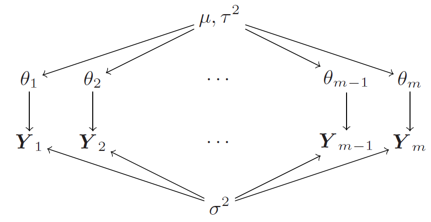
\[ \begin{array}{cl} \text { Within-group model: }\qquad \underline\phi_{j}=\left\{\theta_{j}, \sigma^{2}\right\}, & p\left(y \mid \underline\phi_{j}\right)=\operatorname{N}\left(\theta_{j}, \sigma^{2}\right) \quad \\ \text { Between-group model: }\qquad\underline\psi=\left\{\mu, \tau^{2}\right\}, & p\left(\theta_{j} \mid \underline\psi\right)=\operatorname{N}\left(\mu, \tau^{2}\right) \quad \end{array} \]

The within-group sampling model describes how the data is generated for each group, while the between-group sampling model describes how the group-specific parameters \(\theta_j\) are related to each other through a common mean \(\mu\) and variance \(\tau^2\).

2.1 Priors

\[ \begin{aligned} \sigma^{2} & \sim \operatorname{Inv-Gamma}\left(\nu_{0} / 2, \nu_{0} \sigma_{0}^{2} / 2\right) \\ \tau^{2} & \sim \operatorname{Inv-Gamma}\left(\eta_{0} / 2, \eta_{0} \tau_{0}^{2} / 2\right) \\ \mu & \sim \operatorname{N}\left(\mu_{0}, \gamma_{0}^{2}\right) \end{aligned} \]

Priors for the scale parameters \(\sigma^2\) and \(\tau^2\) are typically set to be Inverse-Gamma, which is a common choice for variance parameters in hierarchical models. The prior for the common mean \(\mu\) (location parameter) is set to be Normal, which allows for semi-conjugacy and simplifies the posterior computations.

2.2 Posterior distributions

We have \(m+3\)-dimensional posterior distribution for \(\left\{\theta_{1}, \ldots, \theta_{m}, \mu, \tau^{2}, \sigma^{2}\right\}\) to estimate. The expression for the posterior distribution simplifies due to the conditional independence structure of the model:

\[ \begin{aligned} & p\left(\theta_{1}, \ldots, \theta_{m}, \mu, \tau^{2}, \sigma^{2} \mid \underline{y}_{1}, \ldots, \underline{y}_{m}\right) \\ &\\ & \propto p\left(\mu, \tau^{2}, \sigma^{2}\right) \times \underbrace{\prod_{j=1}^{m} p\left(\theta_{j} \mid \mu, \tau^{2}\right)}_{\text{Between-group model}} \times \underbrace{p\left(\underline{y}_{1}, \ldots, \underline{y}_{m} \mid \theta_{1}, \ldots, \theta_{m}, \mu, \tau^{2}, \sigma^{2}\right)}_{\text{Within-group model}} \\ & = p\left(\mu, \tau^{2}, \sigma^{2}\right) \times \prod_{j=1}^{m} p\left(\theta_{j} \mid \mu\right) \times p\left(\underline{y}_{1}, \ldots, \underline{y}_{m} \mid \theta_{1}, \ldots, \theta_{m}, \sigma^{2}\right) \\ &\\ & =p(\mu) p\left(\tau^{2}\right) p\left(\sigma^{2}\right)\times \left\{\prod_{j=1}^{m} p\left(\theta_{j} \mid \mu, \tau^{2}\right)\right\}\left\{\prod_{j=1}^{m} \prod_{i=1}^{n_{j}} p\left(y_{i, j} \mid \theta_{j}, \sigma^{2}\right)\right\} . \end{aligned} \]

As usual, there is no closed-form expression for the posterior distribution, but we can derive closed-form expressions for the full conditional distributions of each unknown parameter, which allows us to use Gibbs sampling to approximate the posterior distribution.

We will use the following statement about full conditionals: \[ p(\phi_i\mid \phi_{-i}, y)\quad \propto\quad p(\phi_i, \phi_{-i}\mid y) \]

Exercise: Prove the above statement.

Which means that for each of the parameter, \(\mu\), \(\tau^2\), \(\sigma^2\), and \(\theta_j\)’s, we just need to isolate the terms in the joint posterior that involve the parameter of interest, and we will get the full conditional distribution for that parameter (by recoggnizing the corresponding kernels).

Full conditional distr’n of \(\mu\) and \(\tau^2\)

One can easily verify that the full conditional distributions for \(\mu\) and \(\tau^2\) are given by:

\[ \begin{aligned} \left\{\mu \mid \theta_{1}, \ldots, \theta_{m}, \tau^{2}\right\} &\sim \operatorname{N}\left(\frac{m \bar{\theta} / \tau^{2}+\mu_{0} / \gamma_{0}^{2}}{m / \tau^{2}+1 / \gamma_{0}^{2}},\left[m / \tau^{2}+1 / \gamma_{0}^{2}\right]^{-1}\right) \\ \left\{\tau^{2} \mid \theta_{1}, \ldots, \theta_{m}, \mu\right\} &\sim \operatorname{Inv-Gamma}\left(\frac{\eta_{0}+m}{2}, \frac{\eta_{0} \tau_{0}^{2}+\sum\left(\theta_{j}-\mu\right)^{2}}{2}\right) . \end{aligned} \]

Let’s check our intuition for the full conditional of \(\mu\):

\[ \begin{aligned} p\left(\mu \mid \theta_{1}, \ldots, \theta_{m}, \tau^{2}, \text{data}\right) &\propto p\left(\theta_{1}, \ldots, \theta_{m} , \mu, \tau^{2}, \sigma^{2} \mid \text{data}\right) \\ &\stackrel{\propto}{\small\mu} p(\mu) \times \prod_{j=1}^{m} p\left(\theta_{j} \mid \mu, \tau^{2}\right) \\ &\propto \exp \left\{-\frac{1}{2}\left[\frac{(\mu-\mu_{0})^{2}}{\gamma_{0}^{2}}+\sum_{j=1}^{m} \frac{(\theta_{j}-\mu)^{2}}{\tau^{2}}\right]\right\} \\ \end{aligned} \]

Let’s check our intuition for the full conditional of \(\mu\):

\[ \begin{aligned} \left\{\mu \mid \theta_{1}, \ldots, \theta_{m}, \tau^{2}\right\} &\sim \operatorname{N}\left(\frac{m \bar{\theta} / \tau^{2}+\mu_{0} / \gamma_{0}^{2}}{m / \tau^{2}+1 / \gamma_{0}^{2}},\left[m / \tau^{2}+1 / \gamma_{0}^{2}\right]^{-1}\right) \\ \end{aligned} \]

As a function of \(\mu\), we recognize this as a kernel of a normal distribution!

Exercise: Verify the parameters of the full conditional distribution of \(\mu\).

Exercise: Derive the full conditional distribution of \(\tau^2\) by isolating the terms in the joint posterior that involve \(\tau^2\), and recognizing the kernel of an Inverse-Gamma distribution.

Intuition for the full conditional of \(\tau^2\):

• \(\eta_0 + m\): This is the shape parameter, which is the sum of the prior degrees of freedom and the number of groups. The more groups we have, the more information we have about the variability between groups, which allows us to update our belief about \(\tau^2\). Our sample size for estimating \(\tau^2\) is effectively the number of groups, since \(\tau^2\) captures the variability between group means.

• \(\eta_0 \tau_0^2 + \sum (\theta_j - \mu)^2\): This is the scale parameter, which is the sum of the prior sum of squares and the data sum of squares. The data sum of squares is computed by summing the squared deviations of each group mean \(\theta_j\) from the common mean \(\mu\). This reflects how much variability there is between the group means, which informs our updated belief about \(\tau^2\).

Intuition for the full conditional of \(\mu\): - \(m \bar{\theta} / \tau^2\): This term represents the contribution of the \(m\) group means to the posterior mean of \(\mu\). The average of the group means \(\bar{\theta}\) is weighted by the precision (inverse of variance) of the between-group variability, which is \(m / \tau^2\). This means that if we have more groups or if the variability between groups \(\tau^2\) is smaller, the group means will have a stronger influence on the posterior mean of \(\mu\). - \(\mu_0 / \gamma_0^2\): This term represents the contribution of the prior mean \(\mu_0\) to the posterior mean of \(\mu\). The prior mean is weighted by the precision of the prior distribution, which is \(1 / \gamma_0^2\). This means that if \(\gamma_0^2\) is smaller (indicating stronger belief in the prior mean), the prior mean will have a stronger influence on the posterior mean of \(\mu\). - \(m / \tau^2 + 1 / \gamma_0^2\): This is the precision of the posterior distribution for \(\mu\), which is the sum of the precision from the data (between-group variability) and the precision from the prior. The more groups we have or the smaller \(\tau^2\) is, the more precise our estimate of \(\mu\) will be, and the smaller \(\gamma_0^2\) is, the more precise our prior belief about \(\mu\) will be.

Full conditional of \(\theta_j\)

Using similar intuition as for \(\mu\) and \(\tau^2\), we can derive the full conditional distribution for each \(\theta_j\):

\[ \left\{\theta_{j} \mid y_{1, j}, \ldots, y_{n_{j}, j}, \sigma^{2}\right\} \sim \operatorname{N}\left(\frac{n_{j} \bar{y}_{j} / \sigma^{2}+\mu / \tau^{2}}{n_{j} / \sigma^{2}+1 / \tau^{2}},\left[n_{j} / \sigma^{2}+1 / \tau^{2}\right]^{-1}\right) . \]

Let’s check our intuition for the full conditional of \(\theta_j\):

• \(n_j \bar{y}_j / \sigma^2\): This term represents the contribution of the data from group \(j\) to the posterior mean of \(\theta_j\). The sample mean \(\bar{y}_j\) is weighted by the precision (inverse of variance) of the observations, which is \(n_j / \sigma^2\). This means that if we have more data points in group \(j\) or if the variance \(\sigma^2\) is smaller, the data will have a stronger influence on the posterior mean of \(\theta_j\).

• \(\mu / \tau^2\): This term represents the contribution of the prior mean \(\mu\) to the posterior mean of \(\theta_j\). The prior mean is weighted by the precision of the prior distribution, which is \(1 / \tau^2\). This means that if \(\tau^2\) is smaller (indicating stronger pooling), the prior mean will have a stronger influence on the posterior mean of \(\theta_j\).

Full conditional of \(\sigma^2\)

Finally, the full conditional distribution for \(\sigma^2\) is given by:

\[ \left\{\sigma^{2} \mid \underline{\theta}, \underline{y}_{1}, \ldots, \underline{y}_{m}\right\} \sim \operatorname{Inv-Gamma}\left(\frac{1}{2}\left[\nu_{0}+\sum_{j=1}^{m} n_{j}\right], \frac{1}{2}\left[\nu_{0} \sigma_{0}^{2}+\sum_{j=1}^{m} \sum_{i=1}^{n_{j}}\left(y_{i, j}-\theta_{j}\right)^{2}\right]\right) . \]

Let’s get some intuition for the parameters of the full conditional distribution of \(\sigma^2\):

• \(\nu_0 + \sum_{j=1}^m n_j\): This is the shape parameter, which is the sum of the prior degrees of freedom and the sample sizes across all schools. We use the total number of observations to update our belief about the variance, since the variance is shared across all groups.

• \(\nu_0 \sigma_0^2 + \sum_{j=1}^m \sum_{i=1}^{n_j} (y_{i,j} - \theta_j)^2\): This is the scale parameter, which is the sum of the prior sum of squares and the total data sum of squares. The data sum of squares is computed by summing the squared deviations of each observation from its corresponding group mean \(\theta_j\), across all groups. This reflects how much variability there is in the data around the group means, which informs our updated belief about the variance \(\sigma^2\).

2.3 Data: Math scores in US public schools

The data consists of math scores for 8th grade students from the National Education Longitudinal Study (NELS). The data is organized by school, with each school having its own set of student math scores. We will use this data to fit a hierarchical normal model, where each school’s mean math score is modeled as a random variable drawn from a common distribution.

Here is the data: we can see a large variation in the sample means across schools, and some schools have very small sample sizes, which makes it difficult to estimate their means accurately. This is a perfect setting for applying a hierarchical model, as it allows us to borrow strength across schools and improve our estimates for schools with small sample sizes.

Note how variable the sample means are across schools, especially for schools with small sample sizes. This is a common issue in hierarchical data, and it motivates the use of hierarchical models to borrow strength across groups and improve estimates for groups with limited data.

Setting Parameters for Prior distributions

We nee to set 6 values of the parameters for the prior distributions:

• \(\left(\nu_{0}, \sigma_{0}^{2}\right)\) for \(p\left(\sigma^{2}\right)\),

• \(\left(\eta_{0}, \tau_{0}^{2}\right)\) for \(p\left(\tau^{2}\right)\)

• \(\left(\mu_{0}, \gamma_{0}^{2}\right)\) for \(p(\mu)\).

We are provided with the following guidance for setting these parameters:

Nationwide mean is 50, and nationwide standard deviation is 10:

• \(\mu_0 = 50\) (prior mean for \(\mu\))
• \(\sigma_0^2 = 100\) (expected prior variance for \(\sigma^2\))
• We set \(\nu_0\) to a small value (e.g., \(\nu_0 = 1\)) to make the prior for \(\sigma^2\) weakly informative, allowing the data to have a strong influence on the posterior distribution of \(\sigma^2\).

We desire the mean score \(\mu\) to be between 40 and 60 with high probability:

• This means that \(\gamma_0=5\), so \(\gamma_0^2=25\).

How do we set a prior on the between-group variance \(\tau^2\)? A common Rule of Thumb is the following:

• between group variance \(\tau^2\) should be smaller than the within-group variance \(\sigma^2\).

To make the prior as weakly informative as possible, we can set \(\eta_0=1\) and \(\tau_0^2=100\), which allows for a wide range of values for \(\tau^2\) while still reflecting our belief that the between-group variance is likely to be smaller than the within-group variance.

Gibbs sampling procedure

Given a current state of the unknowns \(\left\{\theta_{1}^{(s)}, \ldots, \theta_{m}^{(s)}, \mu^{(s)}, \tau^{2(s)}, \sigma^{2(s)}\right\}\), a new state is generated as follows:

• sample \(\mu^{(s+1)} \sim p\left(\mu \mid \theta_{1}^{(s)}, \ldots, \theta_{m}^{(s)}, \tau^{2(s)}\right)\);

• sample \(\tau^{2(s+1)} \sim p\left(\tau^{2} \mid \theta_{1}^{(s)}, \ldots, \theta_{m}^{(s)}, \mu^{(s+1)}\right)\);

• sample \(\sigma^{2(s+1)} \sim p\left(\sigma^{2} \mid \theta_{1}^{(s)}, \ldots, \theta_{m}^{(s)}, \underline{y}_{1}, \ldots, \underline{y}_{m}\right)\);

• for each \(j \in\{1, \ldots, m\}\), sample \(\theta_{j}^{(s+1)} \sim p\left(\theta_{j} \mid \mu^{(s+1)}, \tau^{2(s+1)}, \sigma^{2(s+1)}, \underline{y}_{j}\right)\).

Q: Which distribution do we sample from for each of the above steps?

Answer

• For \(\mu^{(s+1)}\), we sample from a Normal distribution, as derived in the full conditional for \(\mu\).
• For \(\tau^{2(s+1)}\), we sample from an Inverse-Gamma distribution, as derived in the full conditional for \(\tau^2\).
• For \(\sigma^{2(s+1)}\), we sample from an Inverse-Gamma distribution, as derived in the full conditional for \(\sigma^2\).
• For each \(\theta_{j}^{(s+1)}\), we sample from a Normal distribution, as derived in the full conditional for \(\theta_j\).

Q: How many parameters do we need to sample in each iteration of the Gibbs sampler?

Answer

In each iteration of the Gibbs sampler, we need to sample \(m + 3\) parameters, where \(m\) is the number of groups (schools) and the additional 3 parameters are \(\mu\), \(\tau^2\), and \(\sigma^2\).

The code for the Gibbs sampling procedure is provided below. We will run the Gibbs sampler for \(S=5000\) iterations, and we will store the samples for \(\theta_j\)’s in a matrix THETA and the samples for \(\mu\), \(\sigma^2\), and \(\tau^2\) in a matrix MST.

#### MCMC approximation to posterior for the hierarchical normal model
## weakly informative priors
nu0<-1  ; s20<-100
eta0<-1 ; t20<-100
mu0<-50 ; g20<-25

## starting values
m<-length(Y) 
n<-sv<-ybar<-rep(NA,m) 
for(j in 1:m) 
{ 
  ybar[j]<-mean(Y[[j]])
  sv[j]<-var(Y[[j]])
  n[j]<-length(Y[[j]]) 
}
theta<-ybar; sigma2<-mean(sv); mu<-mean(theta); tau2<-var(theta)

## setup MCMC
set.seed(1)
S<-5000
THETA<-matrix( nrow=S,ncol=m)
MST<-matrix( nrow=S,ncol=3)

## MCMC algorithm
for(s in 1:S) 
{
  # sample new values of the thetas
  for(j in 1:m) 
  {
    vtheta<-1/(n[j]/sigma2+1/tau2)
    etheta<-vtheta*(ybar[j]*n[j]/sigma2+mu/tau2)
    theta[j]<-rnorm(1,etheta,sqrt(vtheta))
   }
  #sample new value of sigma2
  nun<-nu0+sum(n)
  ss<-nu0*s20;for(j in 1:m){ss<-ss+sum((Y[[j]]-theta[j])^2)}
  sigma2<-1/rgamma(1,nun/2,ss/2)

  #sample a new value of mu
  vmu<- 1/(m/tau2+1/g20)
  emu<- vmu*(m*mean(theta)/tau2 + mu0/g20)
  mu<-rnorm(1,emu,sqrt(vmu)) 

  # sample a new value of tau2
  etam<-eta0+m
  ss<- eta0*t20 + sum( (theta-mu)^2 )
  tau2<-1/rgamma(1,etam/2,ss/2)

  #store results
  THETA[s,]<-theta
  MST[s,]<-c(mu,sigma2,tau2)
} 

mcmc1<-list(THETA=THETA,MST=MST)

MCMC diagnostics

For diagnostic purposes, we will focus on the parameters \(\mu\), \(\sigma^2\), and \(\tau^2\), which are stored in the matrix MST. We will check for convergence using trace plots, compute the effective sample size (ESS) to assess the quality of our MCMC samples, and plot the posterior distributions for these parameters. We use “batched trace plots” to visually assess the stationarity of the MCMC chains for each parameter, and we will also look at the autocorrelation function (ACF) plots to check for any remaining autocorrelation in the samples.

library(coda) # for effectiveSize function
stationarity.plot.sk <- function(x, xlab = "group", ylab = "Value", ...) {
  S <- length(x)
  scan <- 1:S
  ng <- min(round(S / 100), 10)
  group <- S * ceiling(ng * scan / S) / ng

  plot_data <- data.frame(x = x, group = as.factor(group))

  ggplot(plot_data, aes(x = group, y = x, group = group)) +
    geom_boxplot() +
    labs(title = NULL,x = xlab,y = ylab) +
    theme_minimal()
}

stationarity.plot.sk(MST[,1],xlab="iteration",ylab=expression(mu))

stationarity.plot.sk(MST[,2],xlab="iteration",ylab=expression(sigma^2))

stationarity.plot.sk(MST[,3],xlab="iteration",ylab=expression(tau^2))

Parameter	Mean	ESS	MC Error
mu	48.12	3705.9	0.0088
sigma2	84.85	4498.5	0.041
tau2	24.84	2503.5	0.088

Q: How is the MC error computed for each parameter?

The MC error for each parameter is computed as the standard deviation of the MCMC samples for that parameter divided by the square root of the effective sample size (ESS) for that parameter. Mathematically, it can be expressed as: \[ \text{MC Error} = \frac{\text{Standard Deviation of MCMC Samples}}{\sqrt{\text{Effective Sample Size}}}=\frac{SD}{\sqrt{S_{\text{eff}}}} \]

Posterior distributions for \(\mu\), \(\sigma^2\), and \(\tau^2\) can be visualized using density plots. The vertical dashed lines indicate the posterior means for each parameter.

\[ \\[1cm] \]

The ACF plots for \(\mu\), \(\sigma^2\), and \(\tau^2\) show the autocorrelation of the MCMC samples at different lags. Ideally, we want to see that the autocorrelation drops off quickly, indicating that the samples are effectively independent. If there is significant autocorrelation at higher lags, it may indicate that the MCMC chain is not mixing well, and we may need to run the chain for more iterations or consider using a different sampling algorithm.

#### More MCMC diagnostics
par(mfrow=c(1,3))
acf(MST[,1], main=expression("ACF for "*mu))
acf(MST[,2], main=expression("ACF for "*sigma^2))
acf(MST[,3], main=expression("ACF for "*tau^2))

par(mfrow=c(1,1))

Q: Without seeing the effective sample size (ESS) values, which parameters have largest ESS? Smallest ESS? Why?

Answer

• The parameter \(\sigma^2\) has the largest ESS, since the ACF plot for \(\sigma^2\) shows that the autocorrelation drops off more quickly compared to \(\mu\) and \(\tau^2\). This indicates that the samples for \(\sigma^2\) are more effectively independent, leading to a higher ESS.
• The parameter \(\tau^2\) has the smallest ESS, as the ACF plot for \(\tau^2\) shows significant autocorrelation at higher lags, indicating that the samples for \(\tau^2\) are not mixing well and are more correlated, leading to a lower ESS.

For the parameters \(\theta_j\)’s it is tedious to check the trace plots and ACF plots for all \(m\) parameters, so instead we will look at the relationship between the posterior means of \(\theta_j\)’s and their corresponding MC errors and effective sample sizes. This can help us identify if there are any patterns in the MC error or ESS across the different \(\theta_j\)’s, which may indicate issues with convergence or mixing for certain groups.

esTHETA <- effectiveSize(THETA) 
MC.ERROR <-  apply(MST,2,sd)/sqrt( effectiveSize(MST) )

THETA.MC.ERROR <-  apply(THETA,2,sd)/sqrt( effectiveSize(THETA) )
THETA.MC.MEANS <- apply(THETA,2,mean)
par(mfrow=c(1,2))
plot(THETA.MC.MEANS, THETA.MC.ERROR, 
     pch=19, col="skyblue",
     xlab = expression("Posterior mean of " * theta[j]),
     ylab = expression("MC Error of " * theta[j]),
     main = "MC Error vs Mean (THETA_j)")
grid()
plot(THETA.MC.MEANS, esTHETA,
     xlab=expression("Posterior mean of " * theta[j]),
     ylab=expression("Effective sample size of " * theta[j]),
     pch=19, col="navy",
     main = "S_eff vs Mean (THETA_j)")
grid()

Q: Why some of the ESS values are larger than \(S=5000\)?

Answer

The effective sample size (ESS) can be larger than the total number of MCMC iterations (S) when the samples are negatively autocorrelated. Negative autocorrelation can occur when the MCMC chain exhibits a mean-reverting pattern, where the samples alternate around the mean. This can lead to a situation where the samples are more effectively independent than if they were positively autocorrelated, resulting in an ESS that exceeds the total number of iterations.

Shrinkage: sharing information across groups

Shrinkage refers to the phenomenon where the posterior means of the group-level parameters \(\theta_j\)’s are “shrunk” towards the overall mean \(\mu\) compared to the sample means \(ybar_j\). This occurs because the hierarchical model allows for partial pooling of information across groups, which can lead to more accurate estimates for groups with small sample sizes.

More shrinkage occurs for groups with smaller sample sizes, as the model relies more on the overall mean \(\mu\) to inform the estimates for those groups. Conversely, groups with larger sample sizes will experience less shrinkage, as their sample means \(ybar_j\) provide more information about their true means \(\theta_j\). This is clearly visible in the scatter plot of \(ybar_j\) vs. \(\hat{\theta}_j\), where we see that the points corresponding to smaller sample sizes are closer to the overall mean, while those with larger sample sizes are closer to their respective sample means.

Looking closer: data and posterior distributions for two schools

Let us look more closely at the posterior distributions for two schools, one with a small sample size and one with a large sample size. We will plot the posterior density curves for \(\theta_j\) for these two schools, along with the data points (as ticks) and the school sample means (as triangles). We will also include a vertical dashed line to indicate the grand mean \(\mu\).

The light blue curve corresponds to the school with a large sample size (school 46), while the navy curve corresponds to the school with a small sample size (school 82). We can see that the posterior distribution for school 46 is more concentrated around its sample mean, while the posterior distribution for school 82 is more spread out and closer to the grand mean \(\mu\). Also, the posterior mean for school 46 is much closer to its sample mean compared to school 82, since we are quite certain about the true mean for school 46 due to its large sample size, while we are less certain about the true mean for school 82 due to its small sample size, leading to more shrinkage towards the grand mean \(\mu\).

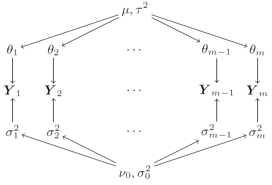
3 Hierarchical modeling of means and variances

A simple extension of the basic hierarchical normal model is to allow for heterogeneity in the variances across groups. In this case, we assume that each group \(j\) has its own variance \(\sigma_j^2\), and we place a prior distribution on these variances. This allows us to model situations where some groups may have more variability than others, which can be important for accurately capturing the underlying data structure.

3.1 Constant vs Non-constant variance

Similarly, we observe shrinkage in the estimates of the variances \(\sigma_j^2\) towards a common value, especially for groups with small sample sizes. Just like for means, the pooling helps to stabilize the estimates of the variances for groups with limited data, while allowing groups with more data to have estimates that are more influenced by their own sample variance.

3.2 Shrinkage

4 Conclusion

That was a lot, wasnt it? This lecture introduced the key concepts of hierarchical modeling through the lens of group comparisons.

Key takeaways:

1. Pooling

Approach	Description	Risk
No pooling	Analyze each group separately (\(\hat\theta_j =\bar{y}_j\))	Risk of Overfitting, especially for small groups
Complete pooling	Ignore group structure and pool all data together (\(\hat\theta_j = \bar{y}\))	Risk of Underfitting, ignores group differences
Partial pooling (hierarchical model)	Model group-level parameters with a common distribution, allowing for shrinkage towards the overall mean	Balances bias and variance; requires MCMC

2. Shrinkage

• Posterior estimates for group-level parameters \(\theta_j\) are always shrunk towards the overall mean \(\mu\).

• The amount of shrinkage depends on

  • Sample size for each group: smaller groups experience more shrinkage (smaller groups have less reliable estimates → borrow more from others).
  • Between-group variance \(\tau^2\): smaller \(\tau^2\) leads to more shrinkage (smaller \(\tau^2\) means groups are more similar → pull toward common mean).
  • Within-group variance \(\sigma^2\): larger \(\sigma^2\) leads to more shrinkage (larger \(\sigma^2\) means noisier data → less trust in group estimates).

3. Power of Hierarchical Models

• With only 2 groups, we must choose the degree of pooling via \(\tau_0^2\).
• With many groups, the data can inform \(\tau^2\), allowing for adaptive pooling. The model automatically determines the amount of pooling.

4. Model Extensions

• Basic hierarchical normal model assumes constant variance across groups.
• We can extend to allow for group-specific variances \(\sigma_j^2\).
• Shrinkage occurs for both means and variances, especially for groups with small sample sizes.

Looking ahead:

Hierarchical modeling extends to:

• regression settings, where we can model group-level effects in a regression framework.
• non-normal data, where we can use hierarchical models for count data, binary data, etc.
• generalized linear mixed models (GLMMs), which allow for both fixed and random effects in a GLM context.