Model selection (or variable selection) is the problem of choosing which predictors to include in a regression model. This is a common problem in applied statistics, as we often have many potential predictors and want to find a parsimonious model that still has good predictive performance.
Frequentist approaches to model selection include:
Forward selection
Backward elimination
Stepwise selection
We will focus on backward elimination.
1.1 WWaFD: Backward Elimination
Here is the general procedure for backward elimination:
Include all predictors.
Find \(\widehat{\underline{\beta}}^{OLS}\).
Choose \(\widehat\beta_i\) with the lowest \(t\)-statistic (i.e. the least siginificant predictor).
Take the corresponding predictor out of the model.
Recompute \(\widehat{\underline{\beta}}^{OLS}\) and repeat until all predictors have \(t\)-statistic above some threshold (e.g. 1.65 for a 10% significance level).
Issues
Common issues with backward elimination include: - It can be computationally expensive, especially when the number of predictors is large, as it requires fitting multiple models. - It can lead to overfitting, as it may select a model that fits the training data well but does not generalize to new data. - It does not account for the uncertainty in the model selection process, which can lead to biased estimates of the coefficients and their standard errors. - It may select more predictors than necessary, leading to a less interpretable model.
1.2 WWaBD: Bayesian Model Selection
From the bayesian perspective, we cannot just select a single model, as we have uncertainty about which model is the best.
Instead, we can compute the posterior distribution over all possible models (i.e. all combinations of predictors) and use this distribution to make predictions. Now, let’s formalize this idea.
Define \(\beta_j=b_j z_j\) for \(j=1,\ldots,p\), in other words: \[
\beta_j=\begin{cases}
b_j & \text{if } z_j=1\\
0 & \text{if } z_j=0
\end{cases}
\]
So the model is: \[
Y_i=(b_1 z_1)X_{i1}+(b_2 z_2)X_{i2}+\ldots+(b_p z_p)X_{ip}+\epsilon_i
\]
In other words, \(z_j\) is an on/off switch for predictor \(j\). We need to find the posterior distribution of \(\underline{b},\underline{z},\sigma^2\) given the data (a \(2p+1\) dimensional distribution).
Q: Write the model for the expected change in oxygen uptake for the following models
\(\underline{z}=(1,0,1,0)\)
\(\underline{z}=(1,1,1,0)\)
Answer
For \(\underline{z}=(1,0,1,0)\), the model is: \[
E[Y_i\mid \underline{X}, \underline{z}=(1,0,1,0)] = b_1 X_{i1} + 0 \cdot X_{i2} + b_3 X_{i3}
\]
For \(\underline{z}=(1,1,1,0)\), the model is: \[
E[Y_i\mid \underline{X}, \underline{z}=(1,1,1,0)] = b_1 X_{i1} + b_2 X_{i2} + b_3 X_{i3}
\]
2 Marginal Posterior
Using the Bayes theorem we can write the posterior distribution as: \[
p(\underline{b},\underline{z},\sigma^2\mid \text{ data})\ \propto\ p(\underline{Y}\mid \underline{X},\underline{b},\underline{z},\sigma^2)\,p(\underline{b},\sigma^2\mid \underline{z})\,p(\underline{z})
\]
Now, for the variable selection problem, we are interested in the marginal posterior distribution of \(\underline{z}\), i.e. \(p(\underline{z}\mid \underline{X},\underline{y})\). In other words, how likely is each model (each combination of predictors) given the data? This is obtained by integrating out \(\underline{b}\) and \(\sigma^2\):
Plugging the above expression for the posterior distribution, we get: \[
\begin{aligned}
p(\underline{z}\mid \underline{X},\underline{y})&\propto\int p(\underline{Y}\mid \underline{X},\underline{b},\underline{z},\sigma^2)\,p(\underline{b},\sigma^2\mid \underline{z})\,p(\underline{z})\,d\underline{b}\,d\sigma^2\\
&=p(\underline{z})\int p(\underline{Y}\mid \underline{X},\underline{b},\underline{z},\sigma^2)\,p(\underline{b},\sigma^2\mid \underline{z})\,d\underline{b}\,d\sigma^2\\
&=p(\underline{z})\,p(\underline{y}\mid \underline{X},\underline{z})
\end{aligned}
\]
Now we need to compute \(p(\underline{y}\mid \underline{X},\underline{z})\), which is the marginal likelihood of the data under model \(\underline{z}\).
Often in practice we can’t compute the denominator, as it requires summing over all \(2^p\) models, which is computationally infeasible for large \(p\). However, we can still compute the numerator for each model and use it to compare models. Comparison is often done using the Bayes factor, which is the ratio of the marginal likelihoods of two models:
Bayes factors can be interpreted as the strength of evidence in favor of one model over another. For example, a Bayes factor of 10 means that the data are 10 times more likely under model \(a\) than under model \(b\). Posterior odds can be interpreted as the probability of one model being true given the data, relative to another model.
4 Dataset: Diabetes
We will investigate the model selection problem using the diabetes dataset, which contains 442 observations and 10 predictors. We enlarge the dataset by including all pairwise interactions between the predictors, resulting in a total of 64 predictors (10 main effects + 45 pairwise interactions + 9 quadratic terms).
Q: Why we do not include the quadratic term for the predictor?
Answer
The predictor is a binary variable (e.g., 0 for male and 1 for female). The quadratic term for a binary variable does not provide any additional information beyond the original variable itself, since \(z^2 = z\) for \(z \in \{0, 1\}\). Therefore, including the quadratic term for the predictor would be redundant and would not contribute to the model’s predictive power.
load("../data/diabetes.RData")head(diabetes$y)
[1] 151 75 141 206 135 97
diabetes$X[1,1:10]
         age          sex          bmi          map           tc          ldl
 0.038075906  0.050680119  0.061696207  0.021872355 -0.044223498 -0.034820763
         hdl          tch          ltg          glu
-0.043400846 -0.002592262  0.019908421 -0.017646125
Note, the predictors has been standardized to have mean 0 and standard deviation 1, and the response has been standardized to have mean 0 and standard deviation 1. This is a common preprocessing step in regression analysis, as it can help with numerical stability and interpretability of the coefficients.
4.1 Marginal likelihood: Likelihood of the data | model
Here is where the \(g\)-prior comes in handy. We can use the \(g\)-prior to compute the marginal likelihood of the data under each model, which is needed to compute the posterior distribution over models. We will skip the technical details of how to compute the marginal likelihood using the \(g\)-prior, but the key point is that it allows us to compute the marginal likelihood in closed form, which is computationally efficient.
\(K\) is a constant that does not depend on the model (i.e. it cancels out when we compute Bayes factors)
\(p_z=\sum_{j=1}^p z_j\) is the number of predictors included in the model (i.e. the number of 1’s in \(\underline{z}\))
\(SSR_g\) is the sum of squared residuals under the \(g\)-prior, which can be computed from the OLS fit of the model.
Interpretation of the marginal likelihood
As \(p_z\) increases, the marginal likelihood decreases due to the \((1+g)^{-p_z/2}\) term, which penalizes more complex models.
As \(SSR_g\) decreases (i.e. the model fits the data better), the marginal likelihood increases due to the \(\frac{1}{(\nu_0\sigma_0^2+SSR_g)^{(\nu_0+n)/2}}\) term, which rewards better fitting models.
So, the competition between these two terms allows us to balance model fit and complexity, which is the essence of model selection.
Exercise: using the above formula, compute the marginal likelihood and the posterior distribution over models for the oxygen uptake dataset we have been working with. Compare the marginal likelihoods of the 5 models we have been working with and interpret the results. Assume that the prior distribution over models is uniform.
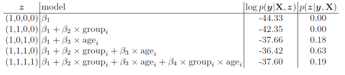
Table: For \(O_2\) uptake example: marginal probabilities of the data under 5 different models
Q: Which model has the highest marginal likelihood? What are the top 3 most likely models according to the posterior distribution over models?
Answer
The model with the highest marginal likelihood is the one with \(z=(1,1,1,0)\), which includes the main effects of , .
The top 3 most likely models according to the posterior distribution over models are:
\(z=(1,1,1,0)\)
\(z=(1,1,1,1)\)
\(z=(1,0,1,0)\)
The Bayesian perspective allows us to use all the models and their corresponding marginal likelihoods to make predictions, rather than just selecting a single model. This is the idea of Bayesian model averaging, which we will discuss in the next section.
4.2 WWaFD: back to Diabetes Dataset
In the Frequentist world in order to assess the performance of a model, we need to evaluate it on a test set that was not used for training. This is because the performance of a model on the training data can be overly optimistic due to overfitting. So, we will split the diabetes dataset into a training set and a test set, fit a full model on the training set, and compute the test error on the test set.
Split the data into 80% and 20% (train + test)
Fit a full model (i.e. a model with all predictors) on the training data
Compute the test error
Predictive performance:\(\frac{1}{100}\sum (y_{test,i}-\widehat{y}_{test,i})^2=\) 0.466 Note, how majority of the coefficients are small. This is a common phenomenon in high-dimensional regression, where many predictors may have little to no effect on the response variable, yet the model includes them. This can lead to overfitting and poor predictive performance on new unseen data. This is one of the reasons why model selection is important, as it allows us to identify a subset of predictors that are most relevant for predicting the response variable. Let’s see how backward elimination performs on this dataset.
The predictive performance is about 10% better than the full model, which is a nice improvement. However, the frequentist world forces us to select a single model, which ignores the uncertainty in the model selection process. In contrast, the Bayesian approach allows us to use all the models and their corresponding marginal likelihoods to make predictions, which can lead to better predictive performance. Let’s see how Bayesian model averaging performs on this dataset.
5 Gibbs Sampling
For this model it seems like it will be tricky to implement a Gibbs sampler, as we have a high-dimensional (\(2p+1\) dimensions) parameter space (\(\underline{z}, \underline{b}, \sigma^2\)) and the posterior distribution is not conjugate.
But, it turns out, we need a Gibbs sampler only for \(\underline{z}\), as we can integrate out \(\underline{b}\) and \(\sigma^2\) to get the marginal likelihood, which is needed to compute the posterior distribution over models. So, we can use a Gibbs sampler to sample from the posterior distribution over \(\underline{z}\).
And then for each sampled \(\underline{z}\), we can compute the posterior distribution over \(\underline{b}\) and \(\sigma^2\) given \(\underline{z}\), which have closed formulas due to the \(g\)-prior.
5.1 Full conditionals for Gibbs sampler
The full conditional for \(z_j\) is defined as \[
p(z_j \mid \underline{z}_{-j}, \underline{X}, \underline{y}) = \frac{p(\underline{y} \mid \underline{X}, \underline{z}_{-j}, z_j) p(z_j \mid \underline{z}_{-j})}{\sum_{z_j} p(\underline{y} \mid \underline{X}, \underline{z}_{-j}, z_j) p(z_j \mid \underline{z}_{-j})}\ \propto\ p(\underline{y} \mid \underline{X}, \underline{z}_{-j}, z_j) p(z_j )
\] Above, \(\underline{z}_{-j}\) denotes the vector \(\underline{z}\) with the \(j\)-th element removed. The numerator can be computed using the formula for the marginal likelihood, and the denominator is just the sum of the numerator over \(z_j \in \{0, 1\}\). The variable \(z_j\) can be sampled from this full conditional distribution, which is a Bernoulli distribution with parameter given by the above expression.
We want to avoid computing the denominator, so we compute the full conditional odds for \(z_j\):
Then, we can sample \(z_j\) from a Bernoulli distribution with parameter \(\frac{odds(z_j)}{1 + odds(z_j)}\).
Exercise: Prove that if a Bernoulli random variable \(Z\) has parameter \(p\), then the odds of \(Z\) being 1 is \(\frac{p}{1-p}\), and the probability of \(Z\) being 1 can be expressed in terms of the odds as \(\frac{odds}{1 + odds}\).
How do we compute the odds? We can compute the marginal likelihoods for \(z_j=1\) and \(z_j=0\) using the formula for the marginal likelihood, which involves computing the sum of squared residuals under the \(g\)-prior for both cases. This allows us to compute the odds without having to compute the denominator, which is computationally efficient.
6 WWaBD: Bayesian Model Averaging
In the plot above we see the prior and posterior inclusion probabilities for each predictor (left plot), as well as the predicted vs actual values for the test set using Bayesian model averaging. The mean squared error of the predictions is also annotated on the plot (MSE=0.406).
Note that only 4 predictors have posterior inclusion probabilities above 0.5, which suggests that these predictors are more likely to be included in the model given the data. But we still have a number of predictors with non-negligible inclusion probabilities, which indicates that there is uncertainty about which predictors are truly relevant for predicting the response variable. This is one of the key advantages of the Bayesian approach, as it allows us to account for this uncertainty in our predictions.
The predictive performance of Bayesian model averaging is better than both OLS and backward elimination, which demonstrates the advantage of using all models and their corresponding marginal likelihoods for prediction, rather than just selecting a single model.
How’s the the prediction for the Bayesian model averaging computed? We run a Gibbs sampler to sample from the posterior distribution over \(\underline{z}\), and for each sampled \(\underline{z}^{(i)}\), we compute the samples \(\underline{\beta}^{(i)}\) from the corresponding posterior distribution. Then, we define
Predictions are then computed as \(\widehat{\underline{y}}^{BMA} = \underline{X}\underline{\beta}^{BMA}\), which is the average of the predictions from all the sampled models, weighted by their posterior probabilities. This is the essence of Bayesian model averaging, which allows us to make predictions that account for the uncertainty in model selection.
Mathematically, we can express the BMA estimate of the coefficients as: \[
\underline{\beta}^{BMA} = E[\underline{\beta}\mid \underline{X}, \underline{y}] = E[\,E[\underline{\beta} \mid \underline{X}, \underline{y}, \underline{z}] \mid \underline{X}, \underline{y}\,]=
E[\underline{\widehat{\beta}}_z \mid \underline{X}, \underline{y}]
\]
We are compute the average of \(\underline{\widehat{\beta}}_z\) (posterior mean of \(\underline{\beta}\) for a given model \(\underline{z}\)) across all models, weighted by the posterior distribution over models \(p(\underline{z} \mid \underline{X}, \underline{y})\). I.e., \[
\underline{\beta}^{BMA} = \sum_{\underline{z}} p(\underline{z} \mid \underline{X}, \underline{y})\cdot \underline{\widehat{\beta}}_z
\] Models with higher probability will contribute more to the BMA estimate, while models with lower probability will contribute less (but still contribute!).
6.1 Collapsed Gibbs sampler
Recall, the full parameter space is \((\underline{z}, \underline{b}, \sigma^2)\), which is high-dimensional.
The regular Gibbs sampler would involve sampling from the full conditionals of \(\underline{z}\), \(\underline{b}\), and \(\sigma^2\).
\[
\text{Ordinary Gibbs sampler:}\qquad
\underline{z}\mid \underline{b}, \sigma^2, \underline{X}, \underline{y} \quad\longrightarrow\quad
\underline{b}\mid \underline{z}, \sigma^2, \underline{X}, \underline{y} \quad\longrightarrow\quad
\sigma^2\mid \underline{z}, \underline{b}, \underline{X}, \underline{y}
\] However, we can integrate out \(\underline{b}\) and \(\sigma^2\) to get the marginal likelihood, which is needed to compute the posterior distribution over models. This allows us to sample directly from the posterior distribution over \(\underline{z}\) without having to sample \(\underline{b}\) and \(\sigma^2\) at each iteration. This is known as a collapsed Gibbs sampler, which can be more efficient in high-dimensional settings.
After each cycle of the collapsed Gibbs, we get a sample of \(\underline{z}\), and we can compute the corresponding \(\underline{\beta}\) and \(\sigma^2\) from their posterior distributions given \(\underline{z}\):
Pseudocode:
for i = 1 to S:
    Sample z^(i) from p(z | X, y) using collapsed Gibbs sampler:
    for j = 1 to p:
        z_j^(i) ~ p(z_j | X, y, z_{-j}^(i))
    Sample σ^2^(i) from p(σ^2 | z^(i), X, y)
    Sample β^(i) from p(β | z^(i), σ^2^(i), X, y)
Figure 1: Collapsed Gibbs sampler over the model indicator vector \(z\), followed by conditional draws of \(\sigma^2\) and \(\beta\).
As \(S\rightarrows \infty\), the samples from the collapsed Gibbs sampler will converge to the posterior distribution over \(\underline{z}\), and the corresponding \(\underline{\beta}\) and \(\sigma^2\) samples will converge to their posterior distributions given \(\underline{z}\):