439/639: SARIMA = Seasonal ARIMA

Author

Dr Sergey Kushnarev

This notebook is based on Chapter 10 of Cryer and Chan, “Time Series Analysis: With Applications in R”.

1 Monthly Carbon Dioxide Levels at Alert, NWT, Canada

1.1 Model specification

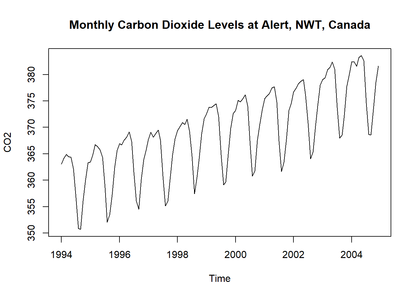
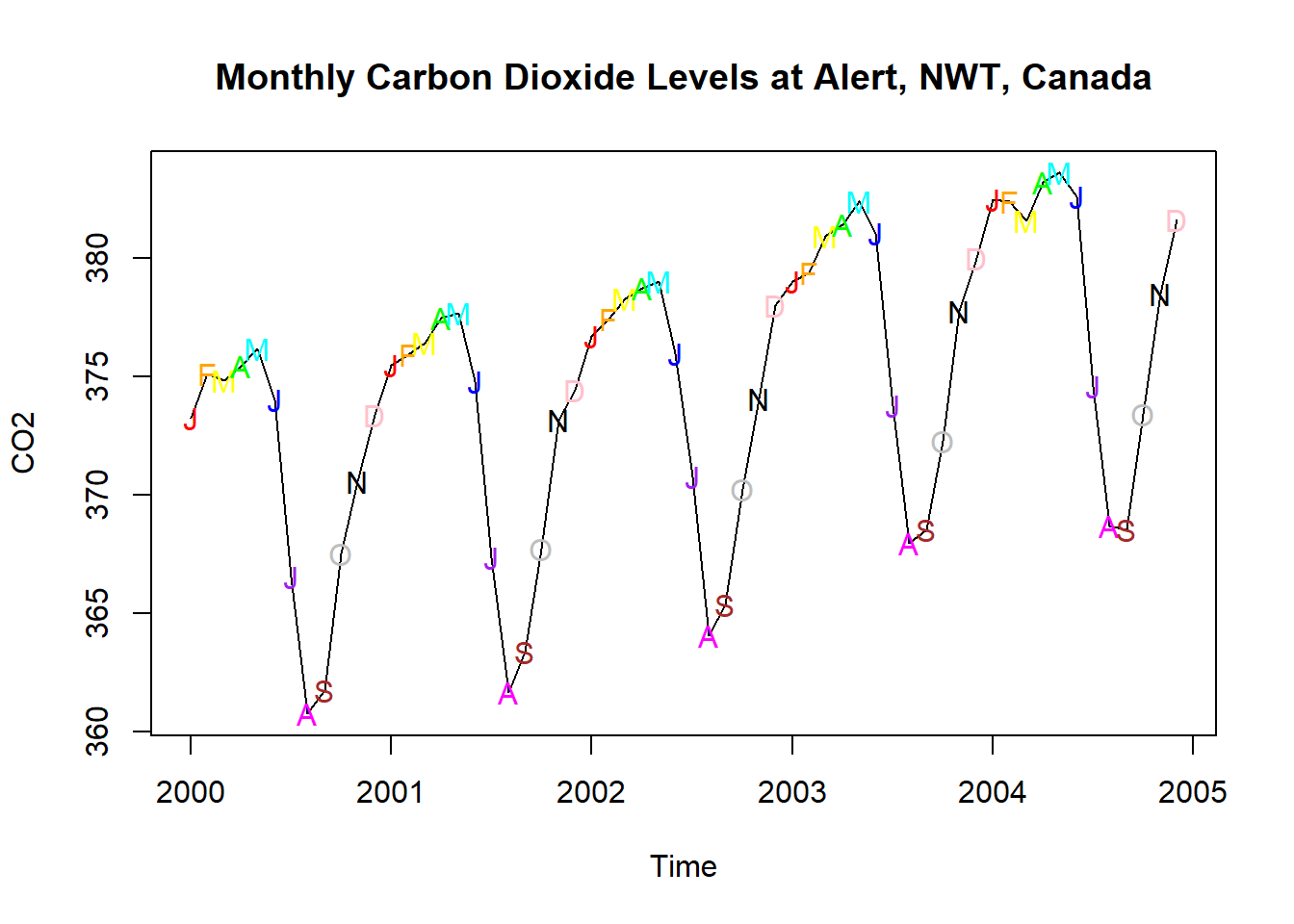
The figure below displays the monthly carbon dioxide levels at Alert, NWT, Canada. The data is available in the TSA package in R. The data is plotted from January 1994 to December 2004. The points are colored according to the month of the year.

Seasonality is more noticable in the second plot, where we colored and labeled the points according to the month of the year.

Code

library(TSA)
data(co2)
plot(co2,ylab='CO2', 
    main='Monthly Carbon Dioxide Levels at Alert, NWT, Canada')

Code

# The points are colored according to the month of the year

# Define colors for each month (12 distinct colors)
month_colors <- c("red", "orange", "yellow", "green", "cyan", 
                  "blue", "purple", "magenta", "brown", "gray", 
                  "black", "pink")
plot(window(co2,start=c(2000,1)),
    ylab='CO2', 
    main ='Monthly Carbon Dioxide Levels at Alert, NWT, Canada')
Month=c('J','F','M','A','M','J','J','A','S','O','N','D')
points(window(co2,start=c(2000,1)),
    pch=Month, col = month_colors[cycle(co2)])

Code

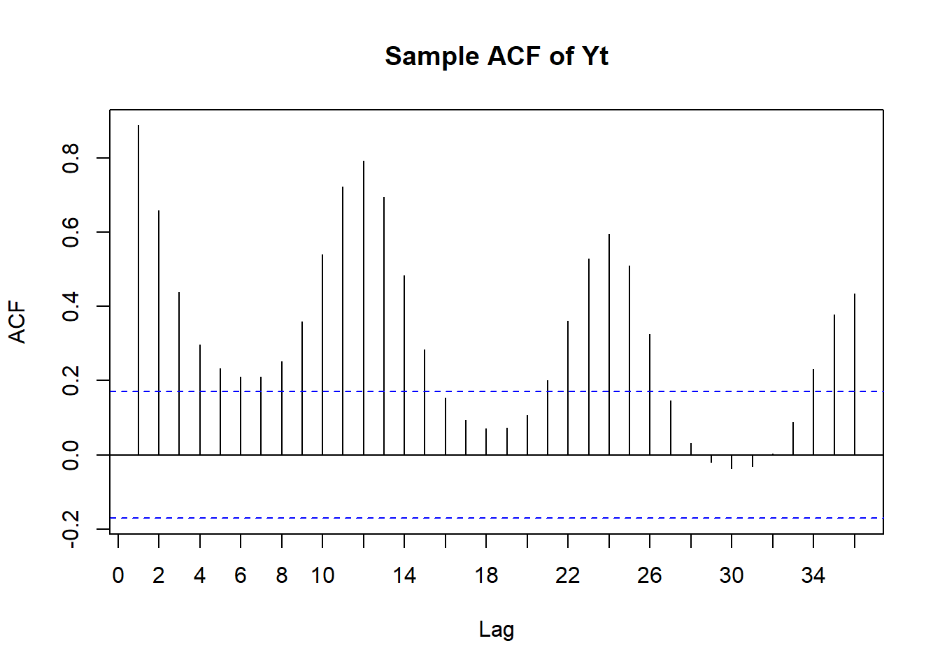
acf(as.vector(co2),lag.max=36, 
    main = 'Sample ACF of Yt',
    xaxp=c(0,36,18))

The sample autocorrelation shows clear signs of seasonality.

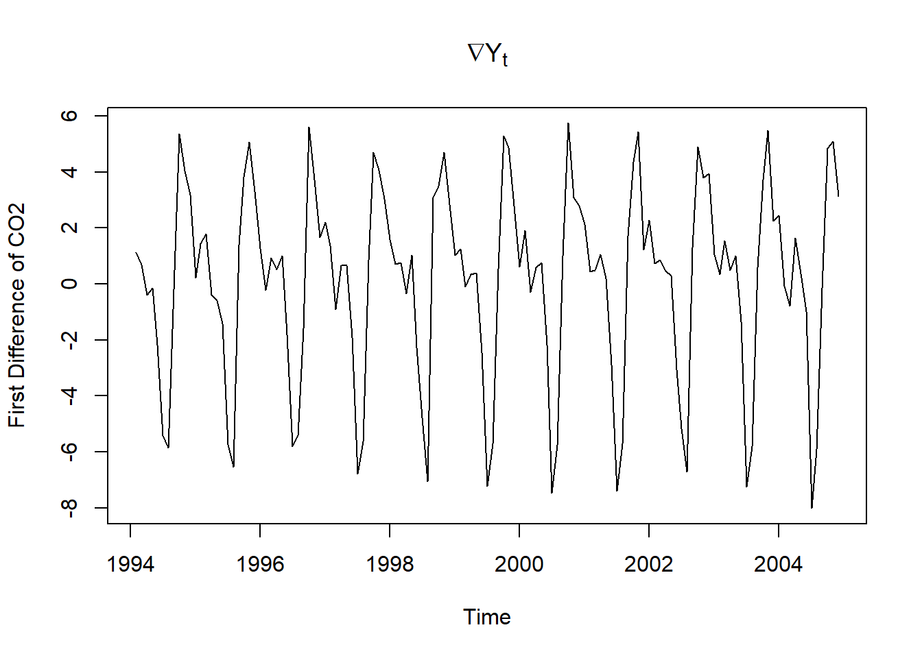
We see a noticeable linear trend in the \(Y_t\) plot, indicating that the data is not stationary. We difference once, \(\nabla Y_t\), and plot the differenced series as well as the corresponding sample ACF.

Code

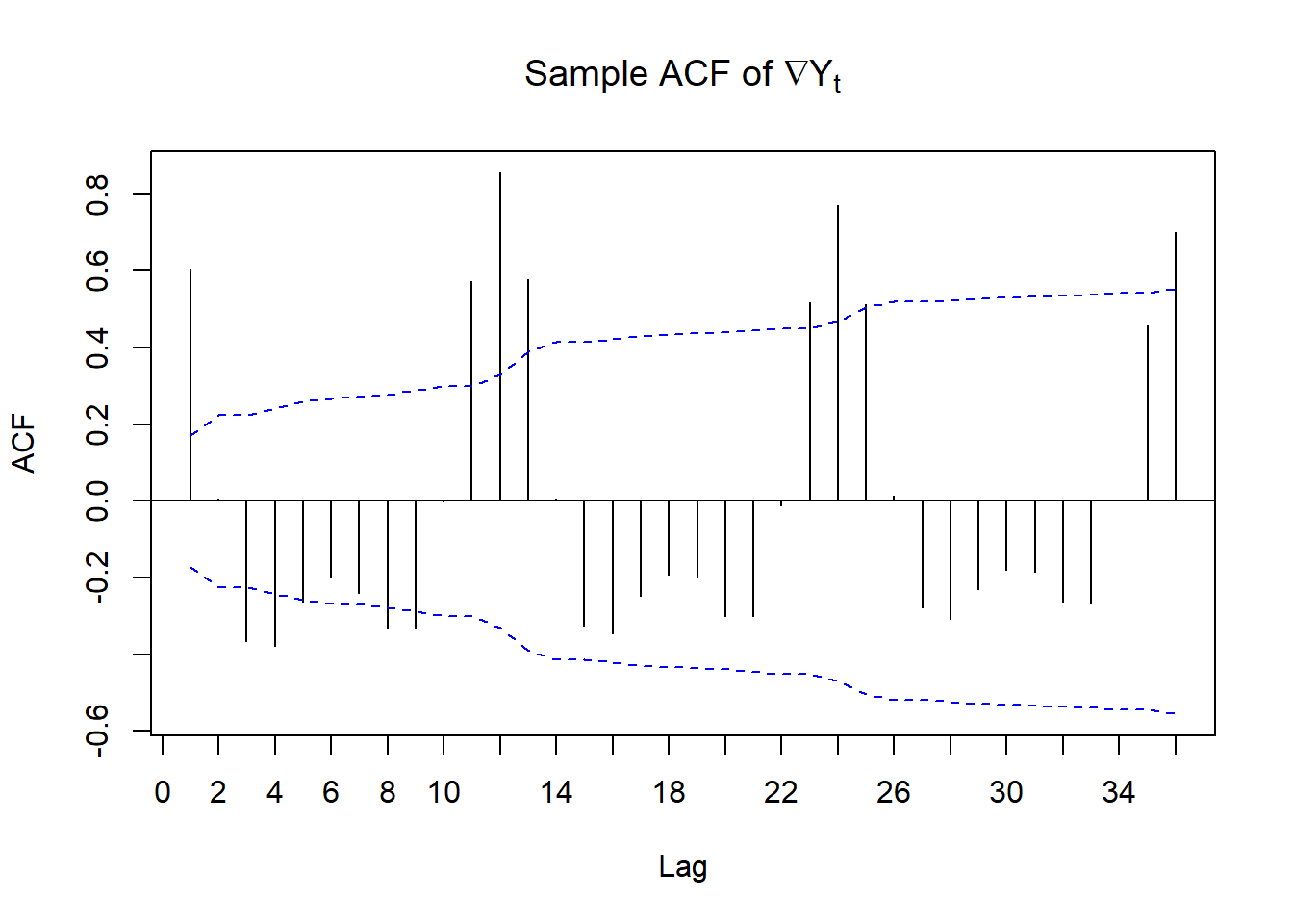
plot(diff(co2),
     ylab='First Difference of CO2',
     xlab='Time',
     main = expression(nabla * Y[t]))

Code

acf(as.vector(diff(co2)),
    lag.max=36,
    ci.type='ma',
    xaxp=c(0,36,18),
    main = expression("Sample ACF of " * nabla * Y[t]))

The general upward trend disappears after the first difference. The ACF of the first difference shows a clear seasonal pattern, with peaks at lags 12, 24, and 36. Perhaps seasonal differencing will bring us to a series that may be modeled parsimoniously. We difference it again at lag 12.

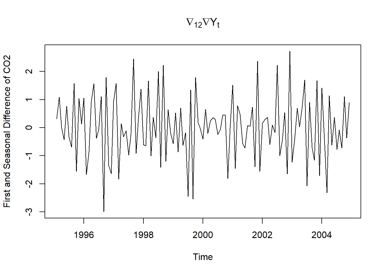
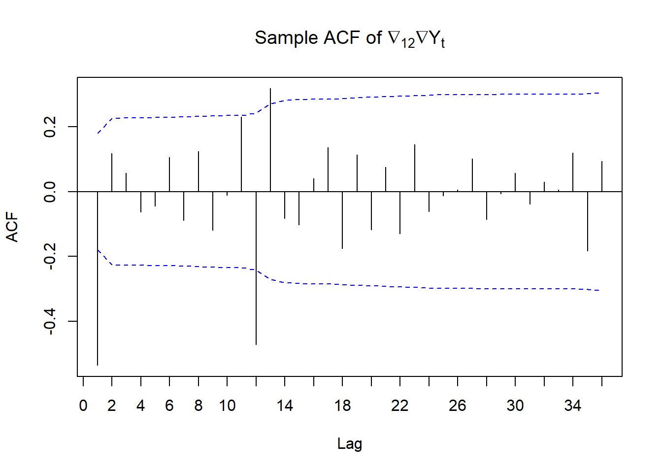
Now we are plotting \(\nabla_{12}\nabla Y_t\) and the corresponding ACF.

Code

plot(diff(diff(co2),lag=12), xlab='Time',
    ylab='First and Seasonal Difference of CO2', 
    main = expression( nabla[12] * nabla * Y[t]))

Code

acf(as.vector(diff(diff(co2),lag=12)),lag.max=36,
    ci.type='ma',xaxp=c(0,36,18), 
    main = expression("Sample ACF of " * nabla[12] * nabla * Y[t]))

Code

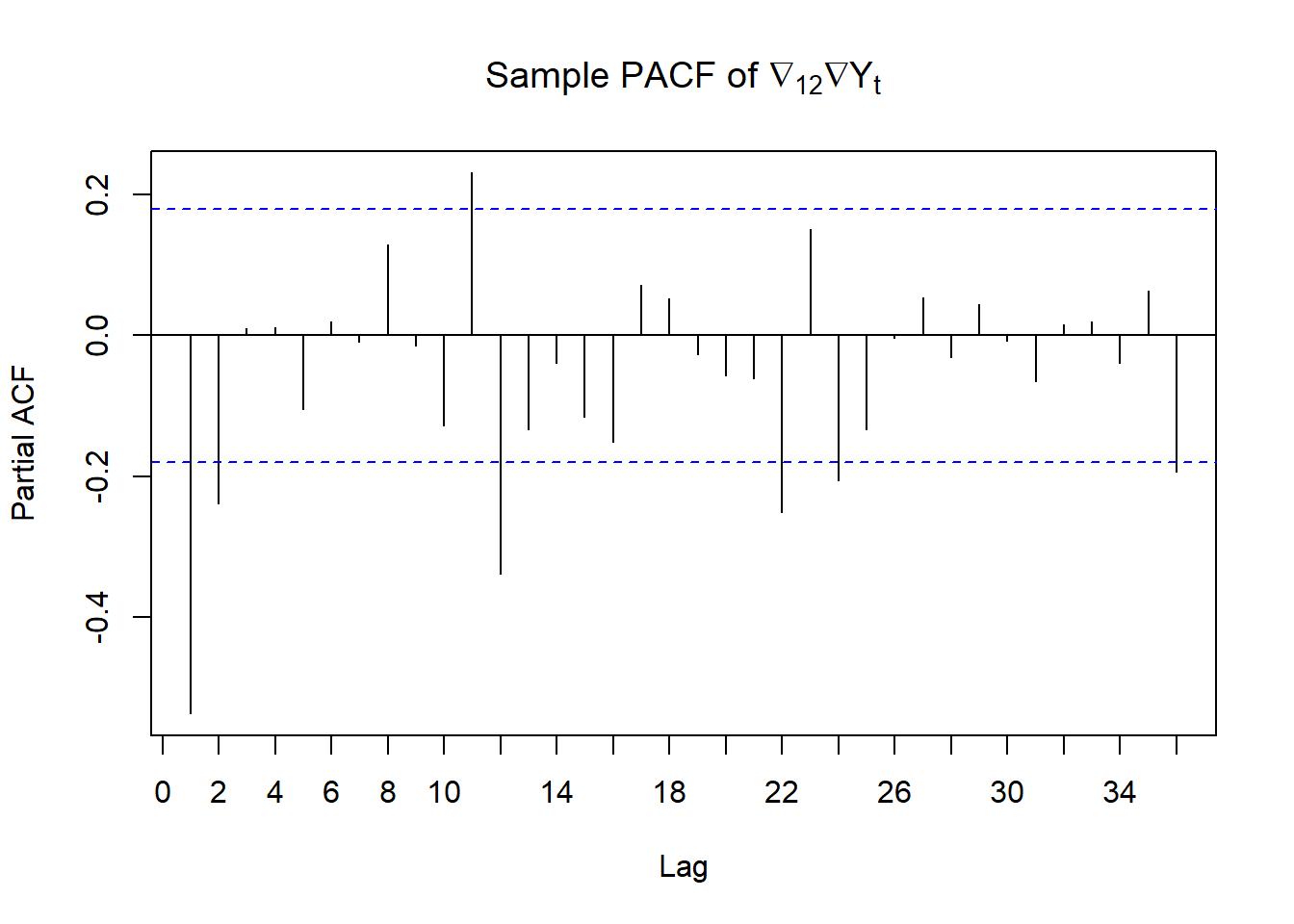
pacf(as.vector(diff(diff(co2),lag=12)),lag.max=36,
    xaxp=c(0,36,18), 
    main = expression("Sample PACF of " * nabla[12] * nabla * Y[t]))

We see significant spikes at lags 1, 12 and 13. We can model this parsimoniously as \(MA(1)\times MA(1)_{12}\). So the original series follows ARIMA\((0,1,1)\times (0,1,1)_{12}\), i.e.

\[ \nabla_{12}\nabla Y_t = e_t-\theta e_{t-1} - \Theta e_{t-12} + \theta\Theta e_{t-13}. \]

1.2 Fitting and Diagnosing the Model

Fitting the model we get the following estimates of the parameters:

Code

m1.co2 <- arima(co2,order=c(0,1,1),
                seasonal=list(order=c(0,1,1),
                period=12))
m1.co2


Call:
arima(x = co2, order = c(0, 1, 1), seasonal = list(order = c(0, 1, 1), period = 12))

Coefficients:
          ma1     sma1
      -0.5792  -0.8206
s.e.   0.0791   0.1137

sigma^2 estimated as 0.5446:  log likelihood = -139.54,  aic = 283.08

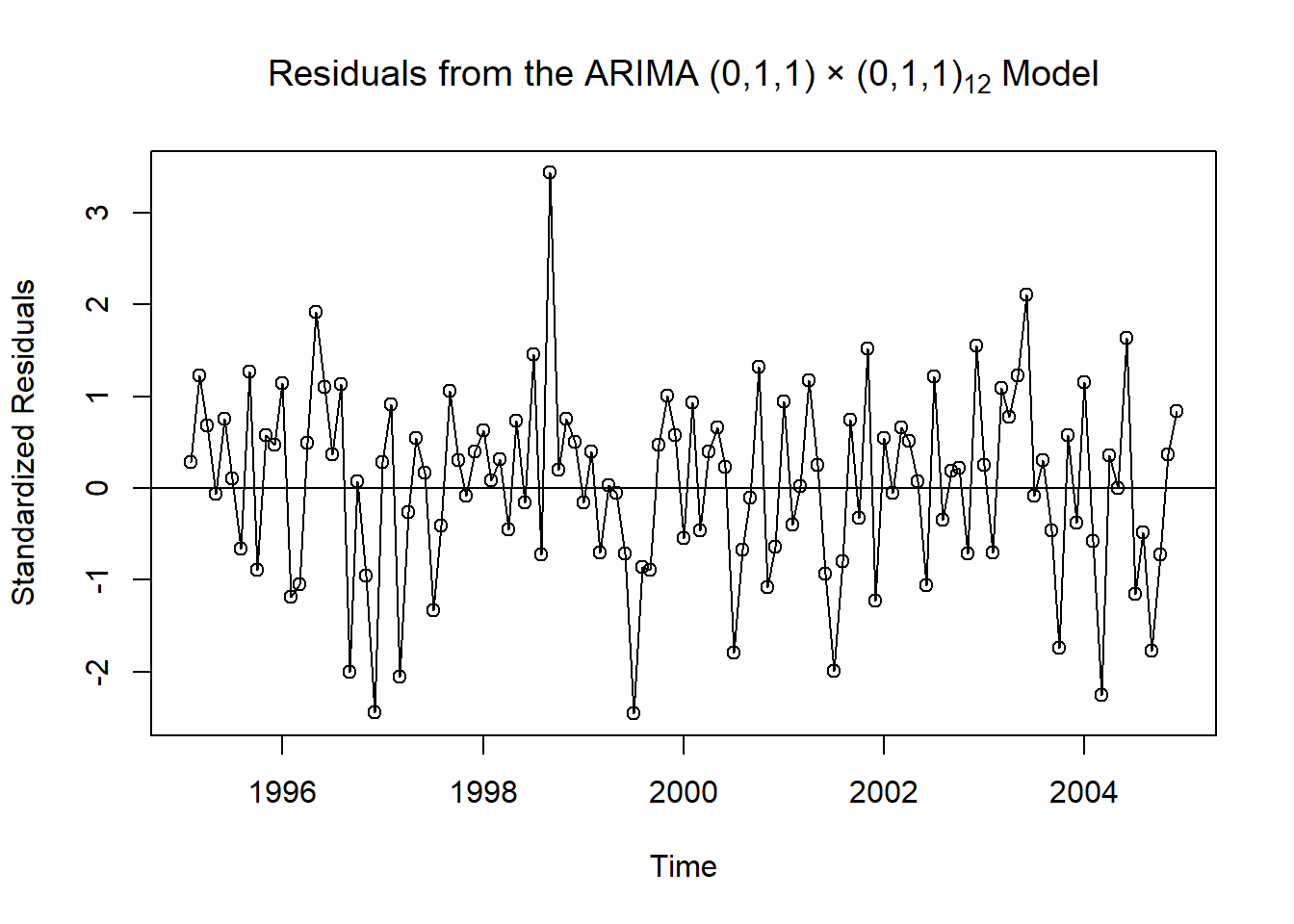
The coefficients are highly significant. We check the residuals of the model. Other than some strange behavior in the middle of the series, this plot does not suggest any major irregularities with the model

Code

plot(window(rstandard(m1.co2),start=c(1995,2)),
    ylab='Standardized Residuals',
    type='o', 
         main = expression("Residuals from the ARIMA" ~
                       "(" * 0 * "," * 1 * "," * 1 * ")" ~
                       "\u00d7" ~
                       "(" * 0 * "," * 1 * "," * 1 * ")"[12] ~
                       "Model"))
abline(h=0)

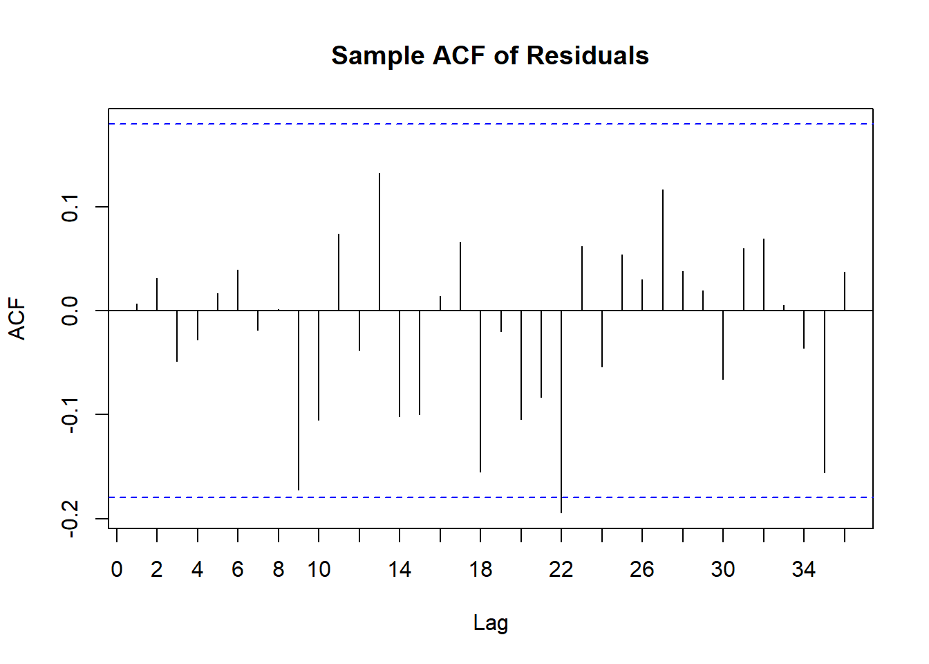
To diagnose further, we plot the sample ACF of the residuals. The only ``statistically significant’’ correlation is at lag 22, and this correlation has a value of only −0.17, a very small correlation. Furthermore, we can’t think of any reasonable interpretation for dependence at lag 22. Finally, we should not be surprised that one autocorrelation out of the 36 displayed is statistically significant. This could easily happen by chance alone. Except for marginal significance at lag 22, the model seems to have captured the essence of the dependence in the series. The Ljing-Box test for the residuals confirms that the residuals are uncorrelated.

Code

acf(as.vector(window(rstandard(m1.co2),start=c(1995,2))),
lag.max=36, main = 'Sample ACF of Residuals',
xaxp=c(0,36,18))

Code

Box.test(window(rstandard(m1.co2),start=c(1995,2)),lag=24,type='Ljung-Box')


    Box-Ljung test

data:  window(rstandard(m1.co2), start = c(1995, 2))
X-squared = 25.587, df = 24, p-value = 0.3745

The histogram, the QQ-plot and the Shapiro-Wilk test for normality of the residuals show that the residuals are nornally distributed.

Code

hist(window(rstandard(m1.co2),start=c(1995,2)),
xlab='Standardized Residuals', main = 'Histogram of Residuals')

Code

qqnorm(window(rstandard(m1.co2),start=c(1995,2)), main = 'QQ-Plot of Residuals')
qqline(window(rstandard(m1.co2),start=c(1995,2)))

Code

shapiro.test(window(rstandard(m1.co2),start=c(1995,2)))


    Shapiro-Wilk normality test

data:  window(rstandard(m1.co2), start = c(1995, 2))
W = 0.98205, p-value = 0.1134

As one additional check, we overfit the model with ARIMA\((0,1,2)\times(0,1,1)_{12}\).

Code

m2.co2 <- arima(co2,order=c(0,1,2),seasonal=list(order=c(0,1,1),
period=12))
m2.co2


Call:
arima(x = co2, order = c(0, 1, 2), seasonal = list(order = c(0, 1, 1), period = 12))

Coefficients:
          ma1      ma2     sma1
      -0.5714  -0.0165  -0.8274
s.e.   0.0897   0.0948   0.1224

sigma^2 estimated as 0.5427:  log likelihood = -139.52,  aic = 285.05

The AIC increased and the new estimated term \(\theta_2\) is not significant, while the other estimated terms have not changed much.

The ARIMA\((0,1,1)\times(0,1,1)_{12}\) model was popularized in the first edition of the seminal book of Box and Jenkins (1976) when it was found to characterize the logarithms of a monthly airline passenger time series. This model has come to be known as the airline model.

1.3 Forecasting

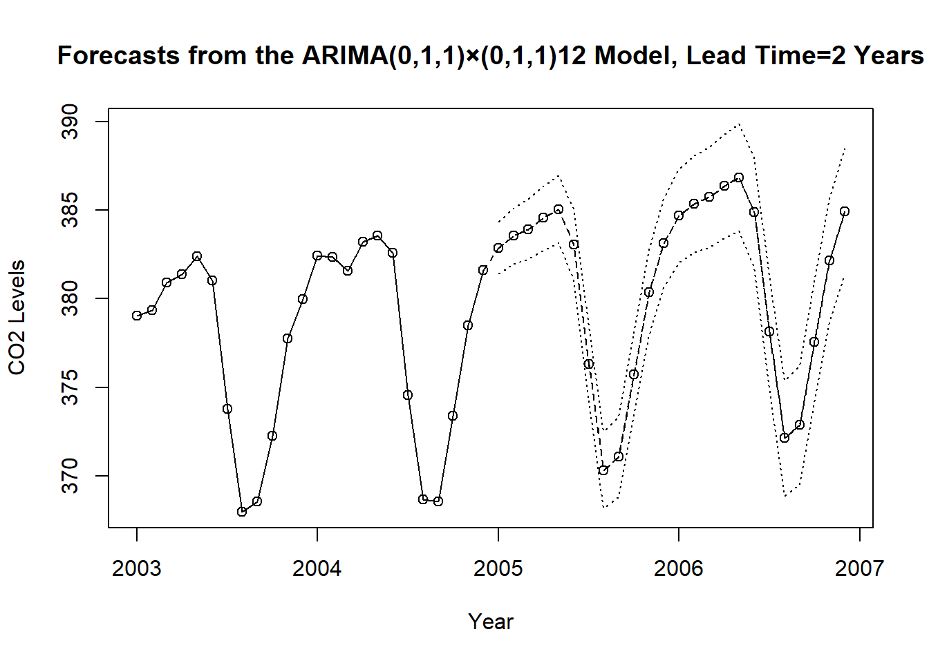
The first plot shows the forecasts and 95% forecast limits for a lead time of two years for the ARIMA\((0,1,1)\times (0,1,1)_{12}\) model that we fit. The last two years of observed data are also shown. The forecasts mimic the stochastic periodicity in the data quite well, and the forecast limits give a good feeling for the precision.

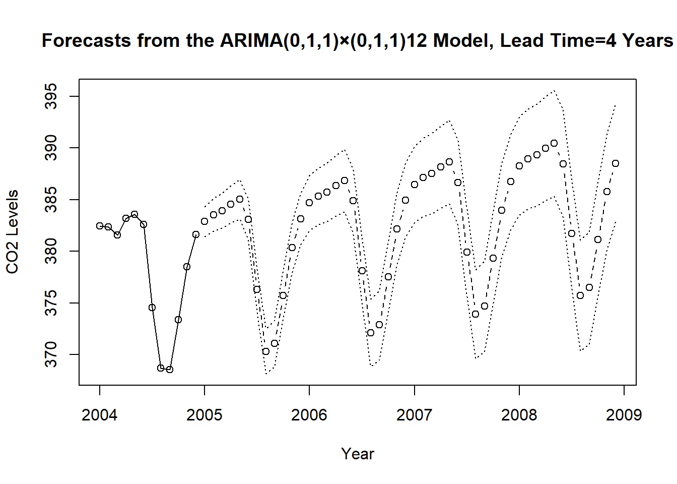
The second plot displays the last year of observed data and forecasts out four years. At this lead time, it is easy to see that the forecast limits are getting wider, as there is more uncertainty in the forecasts.

Code

plot(m1.co2,n1=c(2003,1),n.ahead=24,
    xlab='Year',type='o',ylab='CO2 Levels', 
    main = 'Forecasts from the ARIMA(0,1,1)×(0,1,1)12 Model, Lead Time=2 Years')

Code

plot(m1.co2,n1=c(2004,1),n.ahead=48,
    xlab='Year',type='b', ylab='CO2 Levels', 
    main = 'Forecasts from the ARIMA(0,1,1)×(0,1,1)12 Model, Lead Time=4 Years')

1.4 Summary

Multiplicative seasonal ARIMA models provide an efficient way to model time series whose seasonal tendencies are not as regular as we would have with a deterministic seasonal trend model which we covered earlier. Fortunately, these models are simply special ARIMA models so that no new theory is needed to investigate their properties. We illustrated the special nature of these models with a thorough modeling of an actual time series of CO2 data.