Lecture 7 R notebook: Time Series Plots

Author

Dr Sergey Kushnarev

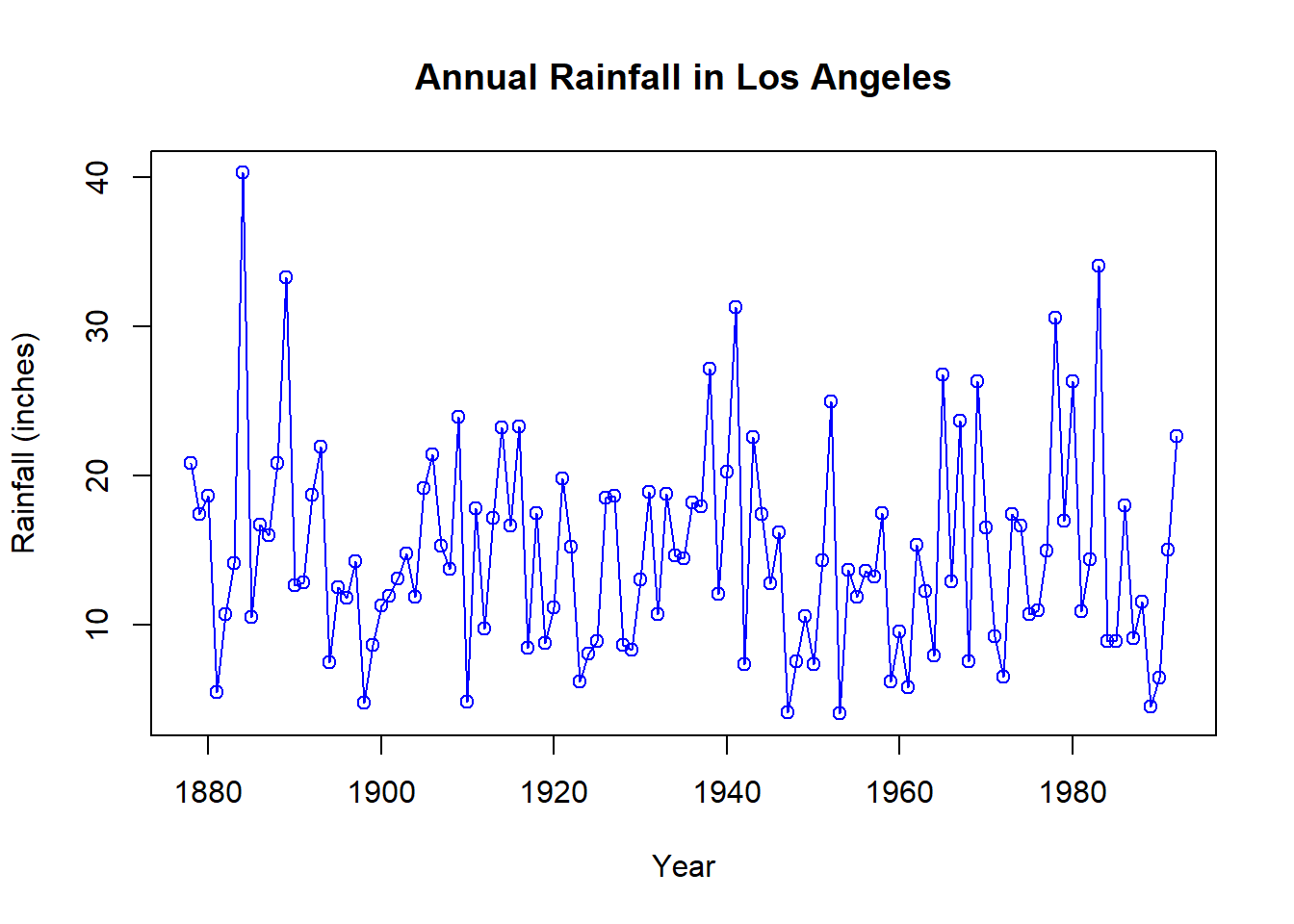
This R notebook is based on a book by Cryer and Chen, “Time Series Analysis: With Applications in R” (2nd edition). We will reproduce some of the plots from the Chapters 1 and 4. These will cover the following topics:

Time series plots
Lag plots
Random walk
ACF and time series plots for: MA(1), MA(2), AR(1), AR(2), ARMA(1,1)

0.1 Los Angeles Annual Rainfall

Code

#install.packages("TSA")
library(TSA)
data(larain)
plot(larain, type = "o", col = "blue", xlab = "Year", ylab = "Rainfall (inches)", 
     main = "Annual Rainfall in Los Angeles")

Code

# Lag plot
plot(y=larain,
     x=zlag(larain),
     ylab='Inches',
     xlab='Previous Year Inches',
     col = 'blue',
     main='Lag Plot of Annual Rainfall in Los Angeles')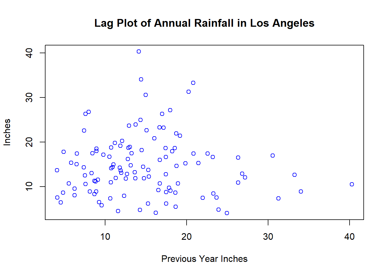

0.2 Color Property from Chemical Process

Code

data(color)
plot(color,
     ylab='Color Property',
     xlab='Batch',
     type='o',
     main='Color Property from Chemical Process',
     col = 'blue')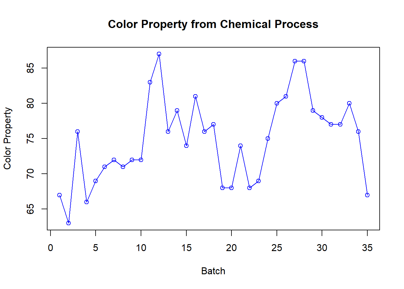

Code

# Lag plot
plot(y=color,
     x=zlag(color),
     ylab='Color Property',
     xlab='Previous Batch Color Property', 
     col = 'blue',
     main='Lag Plot of Color Property from Chemical Process')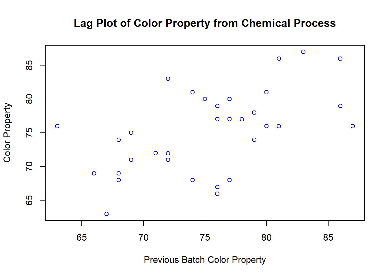

0.3 Hare Abundance in Canada

Code

data(hare)
plot(hare,
     ylab='Abundance',
     xlab='Year',
     type='o', col = 'blue',
     main='Hare Abundance in Canada')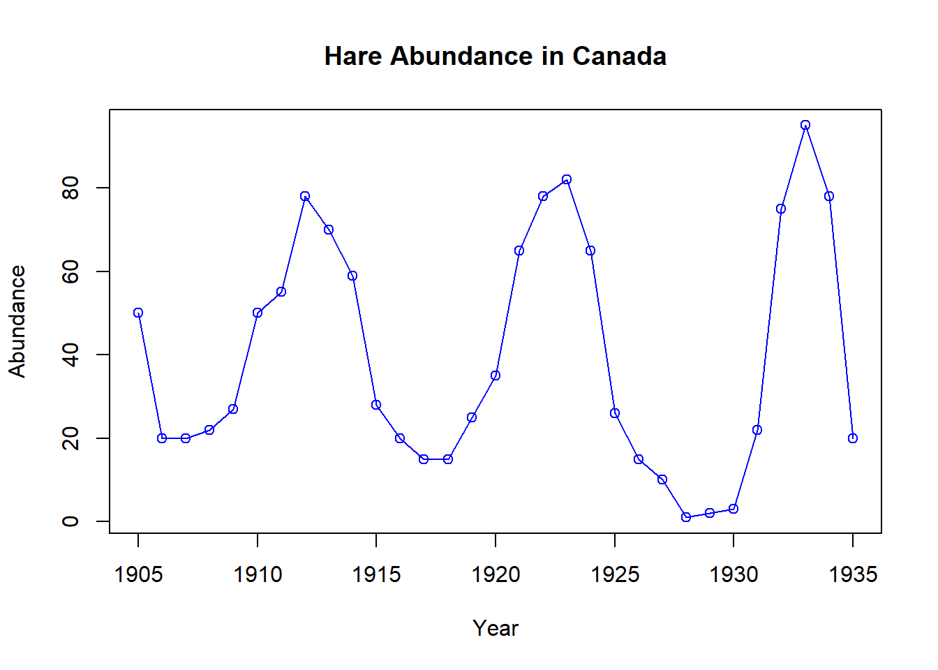

Code

# Lag plot
plot(y=hare,
     x=zlag(hare),
     ylab='Abundance',
     xlab='Previous Year Abundance', 
     col = 'blue',
     main='Lag Plot of Hare Abundance in Canada')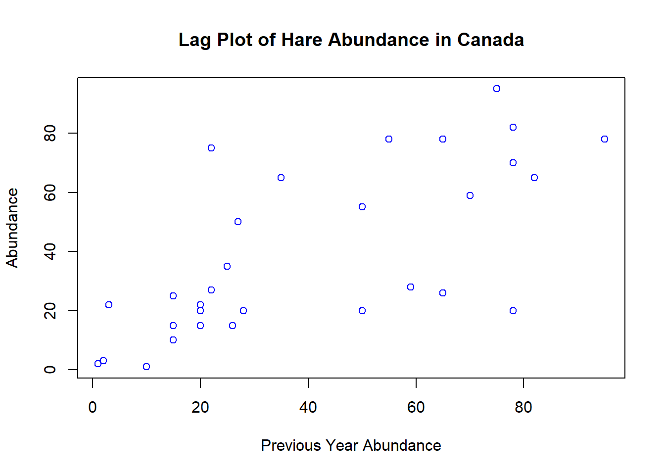

0.4 Average Monthly Temperatures, Dubuque, Iowa

Code

# Average Monthly Temperatures, Dubuque, Iowa
data(tempdub) 
plot(tempdub,
     ylab='Temperature',
     type='o', 
     col = 'blue',
     xlab='Month',
     main='Average Monthly Temperatures, Dubuque, Iowa')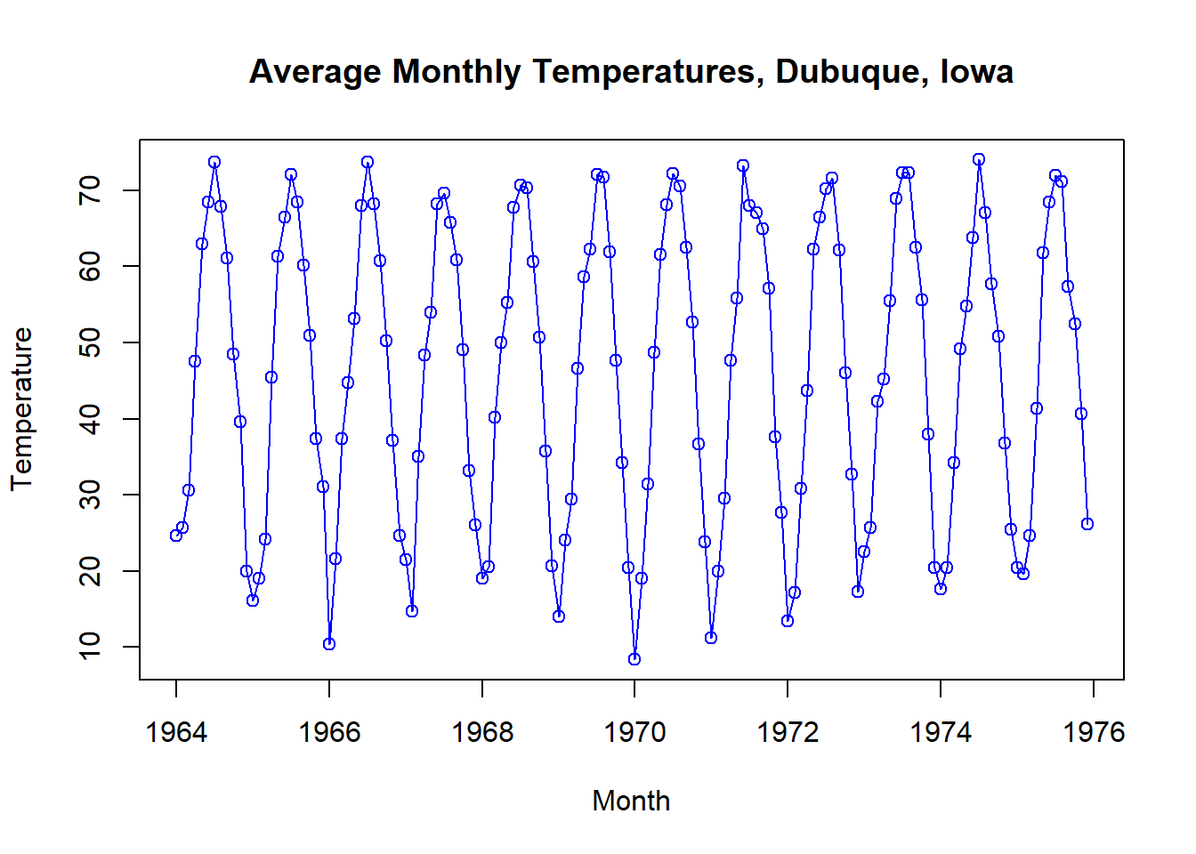

Code

# Lag plot
plot(y=tempdub,
     x=zlag(tempdub),
     ylab='Temperature',
     xlab='Previous Month Temperature', 
     col = 'blue',
     main='Lag Plot of Average Monthly Temperatures, Dubuque, Iowa')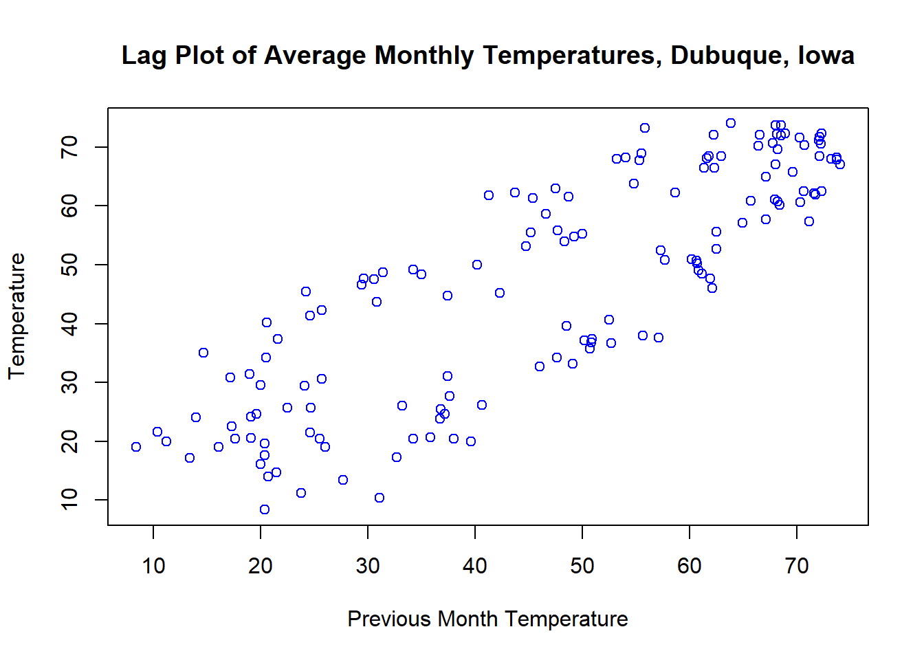

0.5 Oil Filter Sales

Code

data(oilfilters) 
oilfilters

      Jan  Feb  Mar  Apr  May  Jun  Jul  Aug  Sep  Oct  Nov  Dec
1983                               2385 3302 3958 3302 2441 3107
1984 5862 4536 4625 4492 4486 4005 3744 2546 1954 2285 1778 3222
1985 5472 5310 1965 3791 3622 3726 3370 2535 1572 2146 2249 1721
1986 5357 5811 2436 4608 2871 3349 2909 2324 1603 2148 2245 1586
1987 5332 5787 2886 5475 3843 2537

Code

plot(oilfilters,
     type='o',
     ylab='Sales',
     xlab='Month',
     main='Oil Filter Sales',
     col = 'blue')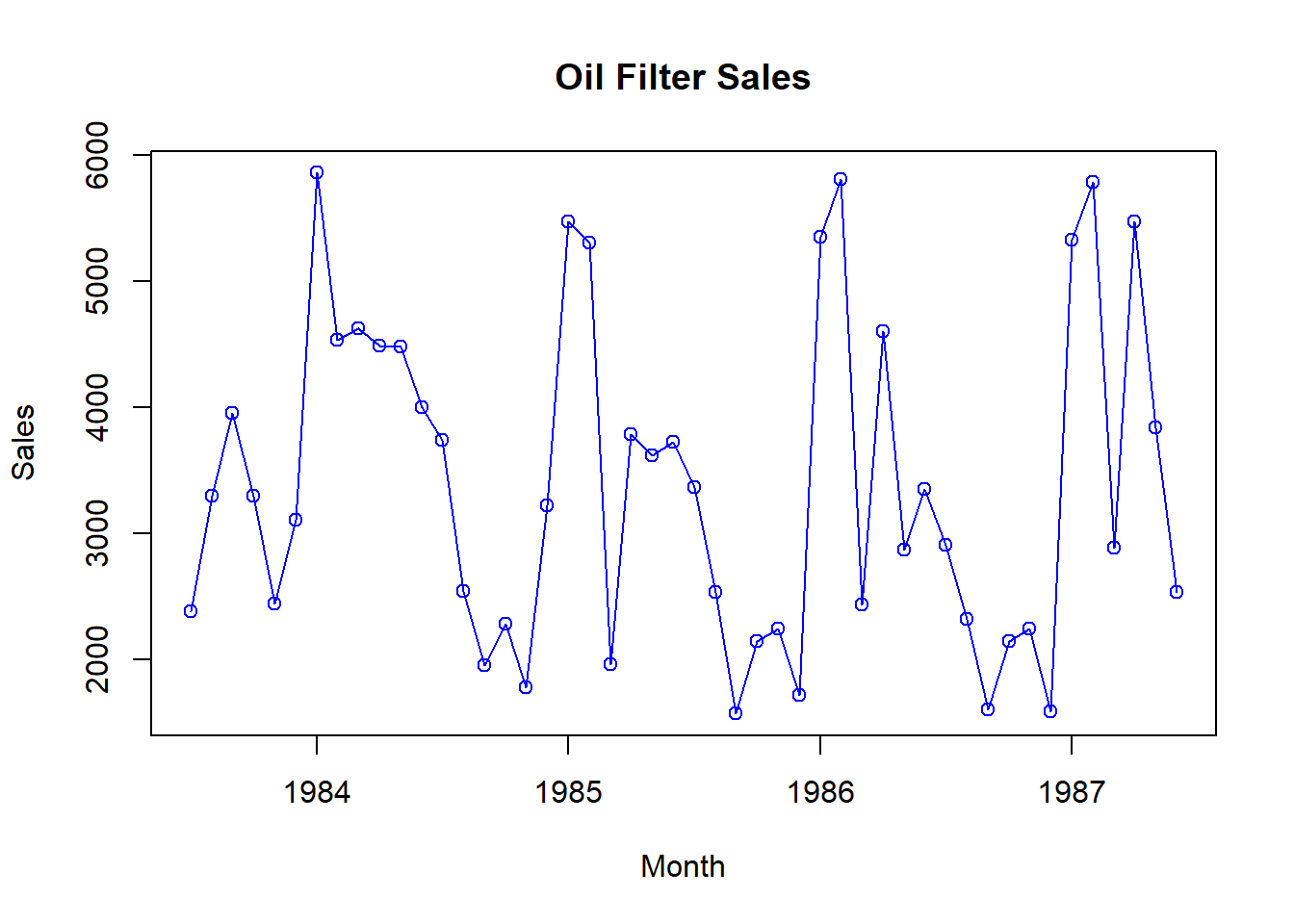

Code

plot(oilfilters,
     type='l',
     ylab='Sales', 
     col = 'blue',
     xlab='Month',
     main='Oil Filter Sales')
points(y=oilfilters,
      x=time(oilfilters),
      pch=as.vector(season(oilfilters)),
      col = 1:4)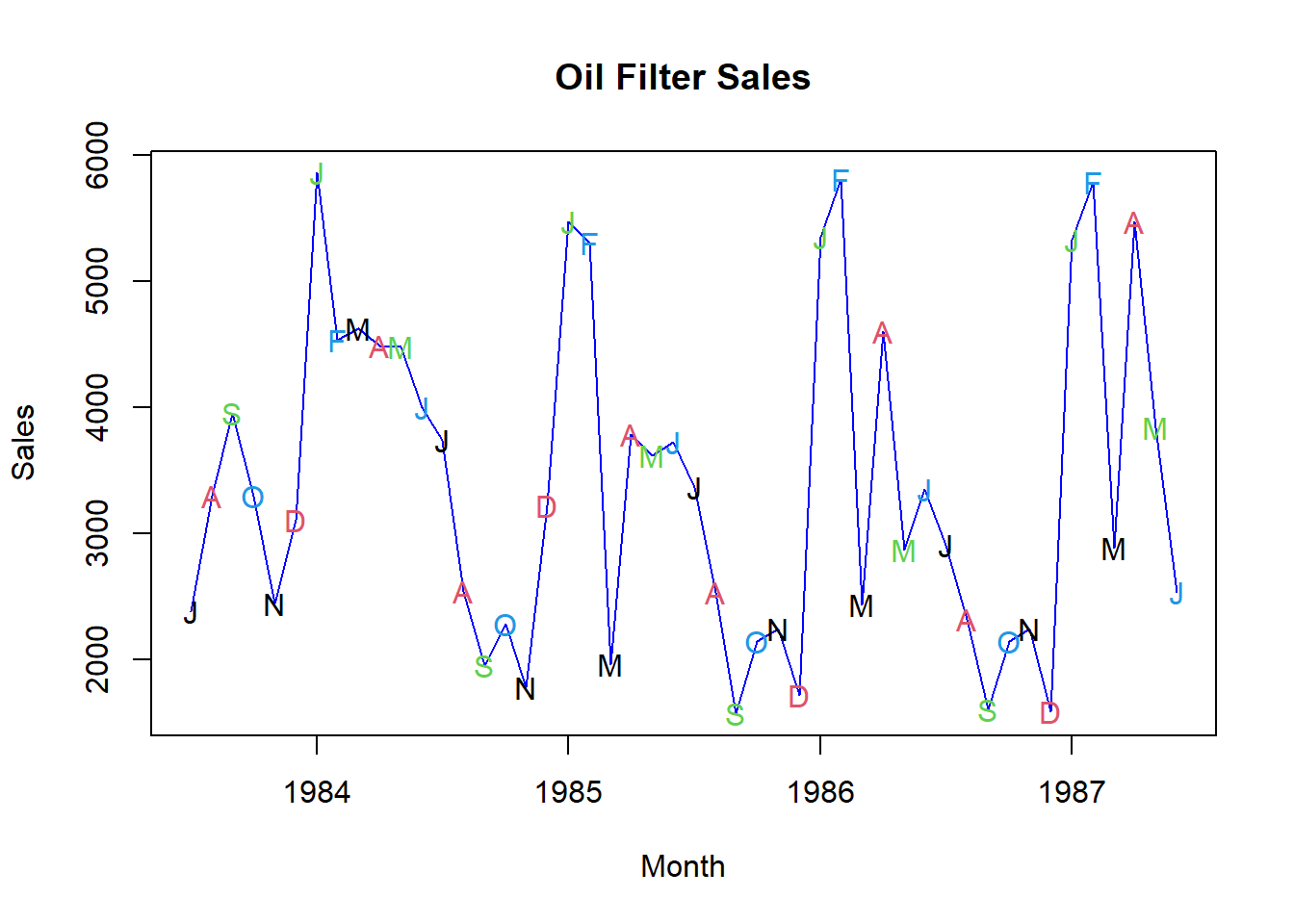

0.6 Random Walk

Code

set.seed(439)
data(rwalk) # rwalk contains a simulated random walk
rw2 <- cumsum(rnorm(length(rwalk)))
rw3 <- cumsum(rnorm(length(rwalk)))
# plot all three series
plot(rwalk,
     type='o',
     ylab='Random Walk', 
     col = 'blue')
points(rw2,
       type='o',
       ylab='Random Walk', 
       col = 'red')
points(rw3,
       type='o',
       ylab='Random Walk', 
       col = 'green')
legend('topleft',
       legend=c('rwalk','rw2','rw3'),
       col=c('blue','red','green'),
       lty=1)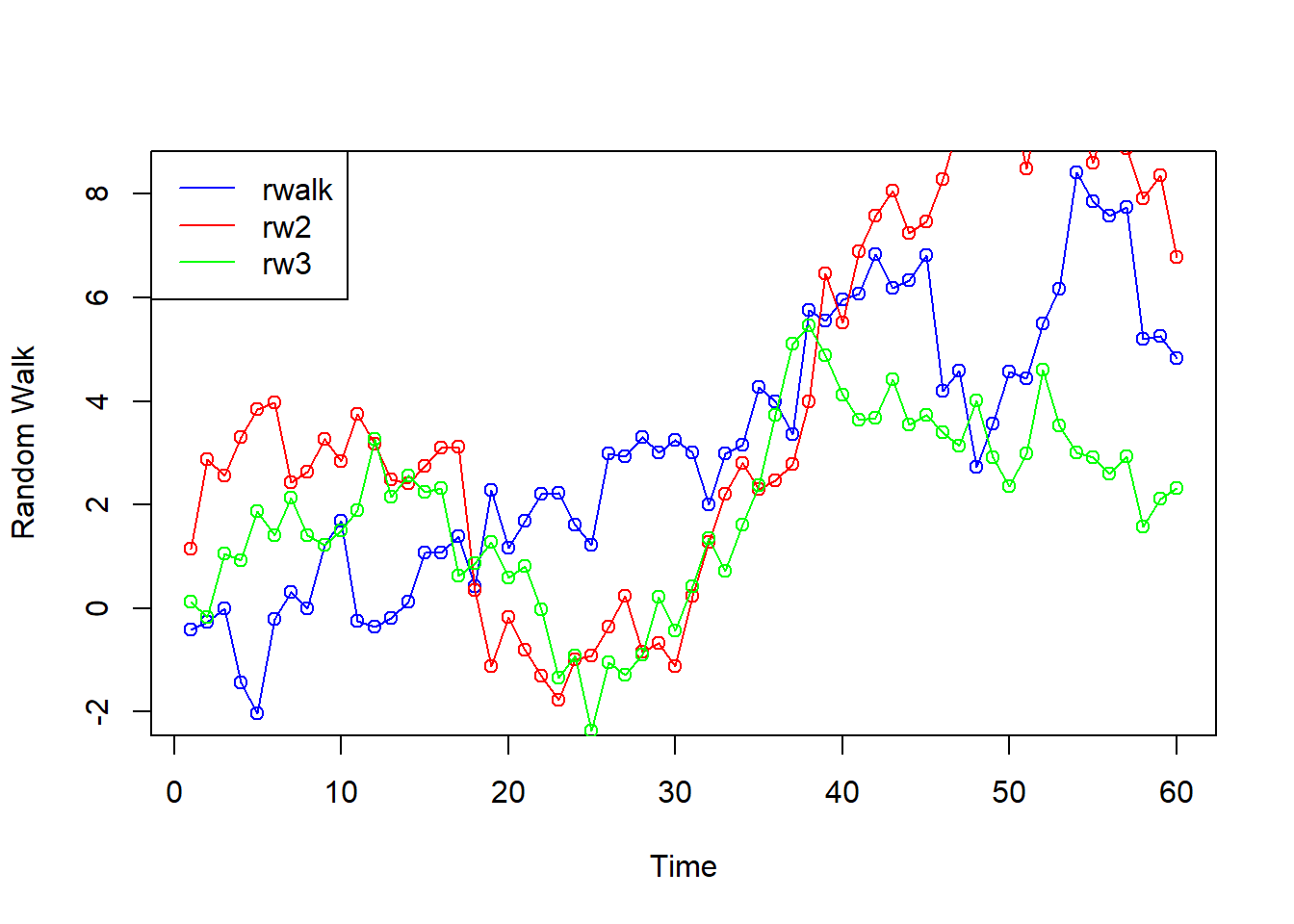

1 Chapter 4

1.1 MA(q) processes

Code

# Lag 1 autocorrelation for MA(1) model
theta <- seq(-10,10,by=0.1)
rho1 <- -theta/(1+theta^2)
plot(theta,rho1,
     type='l',
     ylab='rho(1)',
     xlab='theta',
     col = 'blue',
     main='Lag 1 Autocorrelation for MA(1) model')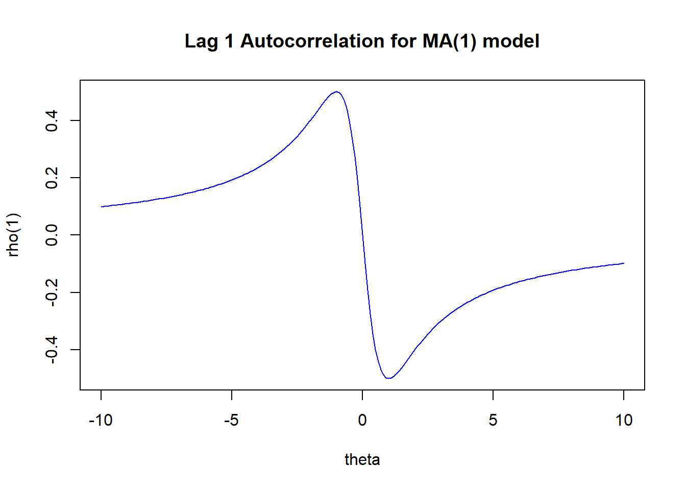

Code

# Lag 1 autocorrelation for MA(1) model
theta1 <- theta[theta >= -1 & theta <= 1]
rho11 <- -theta1/(1+theta1^2)
plot(theta1,rho11,
     type='l',
     ylab='rho(1)',
     xlab='theta',
     col = 'blue',
     main='Lag 1 Autocorrelation for MA(1) model')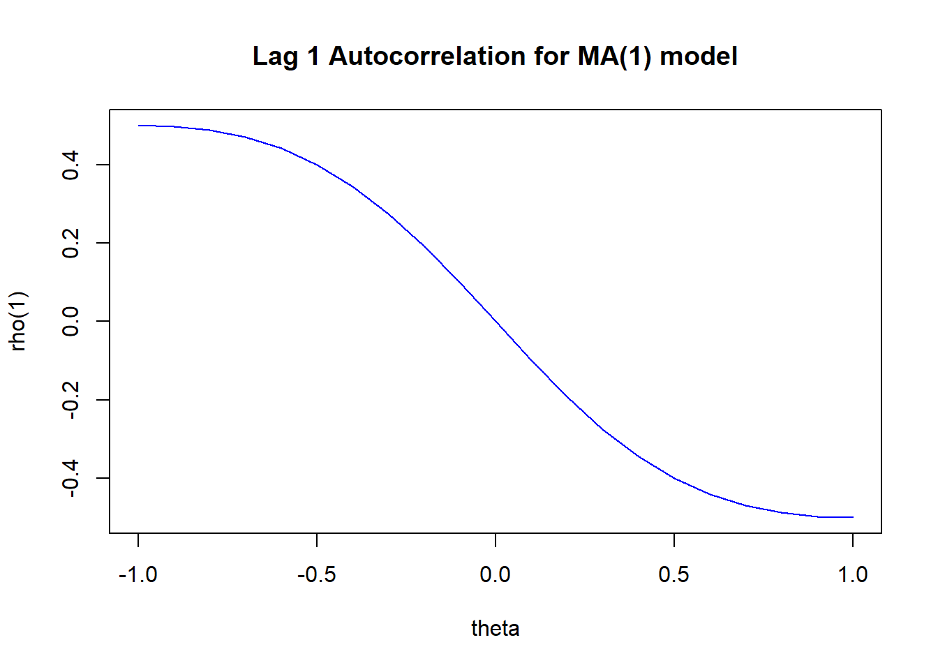

Code

# Time plot of an MA(1) process with theta = -0.9
data(ma1.2.s)
plot(ma1.2.s,
     ylab=expression(Y[t]),
     type='o', 
     col = 'blue',
     xlab='Time',
     main='MA(1) process with theta = -0.9')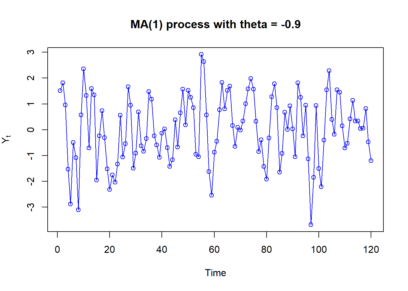

Code

par(mfrow = c(1, 2), mar = c(4, 4, 2, 2), oma = c(0, 0, 5, 0))
# Lag plot Yt vs Y_(t-1) for an MA(1) process with theta = -0.9
# with the lowess smoother
plot_lag_lowess <- function(ts_data, num_lags, main_title = "Lag Plots with LOWESS Smoother") {
  par(mfrow = c(ceiling(num_lags / 2), 2),  # Arrange plots in a grid
      mar = c(4, 4, 2, 2),  # Margins: (bottom, left, top, right)
      oma = c(1, 1, 2, 1),
      pty = 's')  # Outer margins for better spacing

  for (i in 1:num_lags) {
    x <- ts_data[1:(length(ts_data) - i)]  # Lagged values
    y <- ts_data[(i + 1):length(ts_data)]  # Corresponding Y_t values

    # Plot scatter plot
    plot(x, y, pch = 'o', col = 'blue',
         #main = paste('Lag Plot Y_t vs Y_(t-', i, ')'),
         xlab = paste('Y_(t-', i, ')', sep = ''),
         ylab = 'Y_t',
         asp = 1)

    # Add LOWESS fitted line
    lines(lowess(x, y, f = 2/3), col = 'red', lwd = 2)

    # Add main title across all subplots
     mtext(main_title, outer = TRUE, cex = 1.5, font = 2)
  }
 # Reset plotting layout and default shape
  par(mfrow = c(1, 1), pty = "m")
}

plot_lag_lowess(ma1.2.s, num_lags = 4)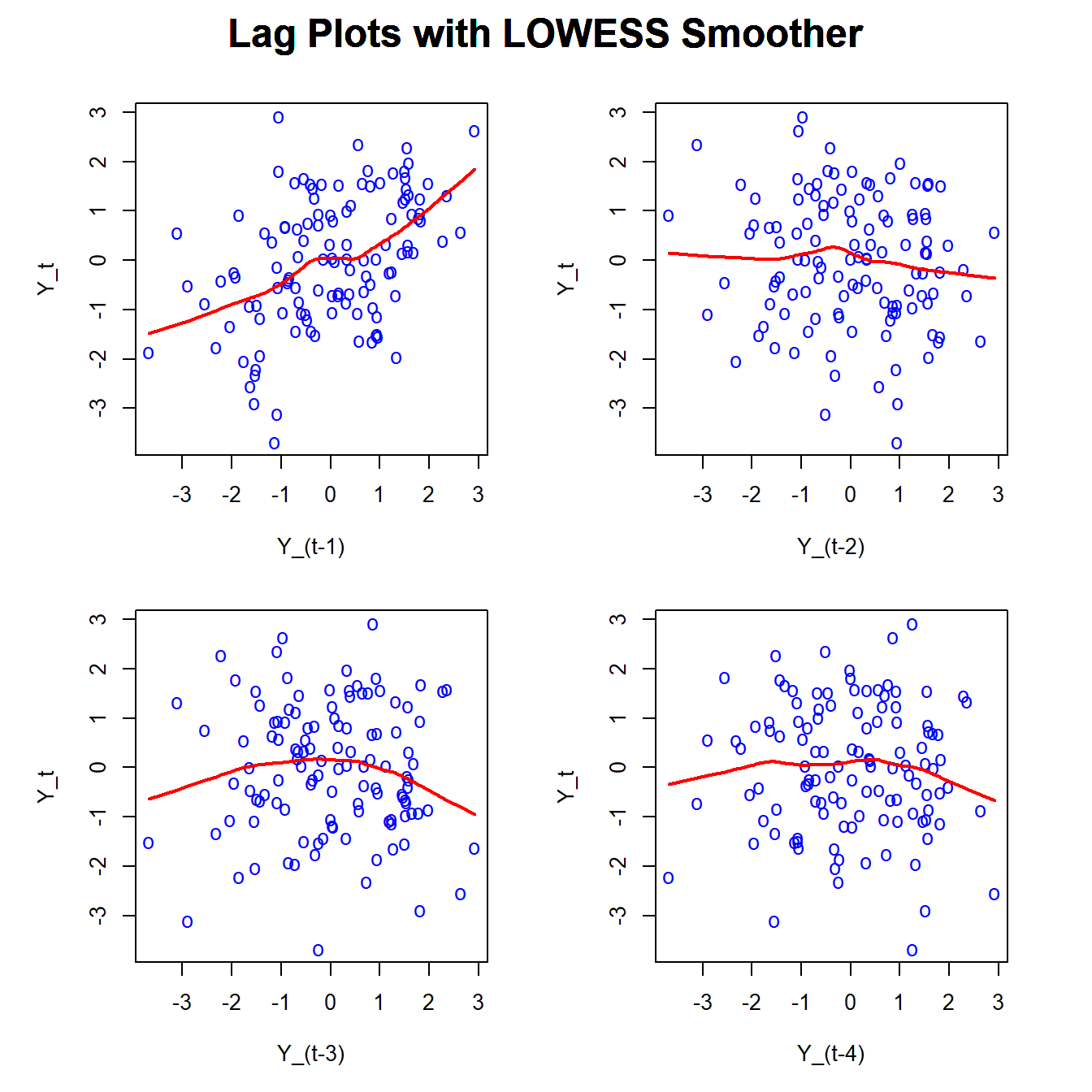

Code

# Time plot of an MA(1) process with theta = +0.9
data(ma1.1.s)
plot(ma1.1.s,
     ylab=expression(Y[t]),
     type='o', 
     col = 'blue',
     xlab='Time',
     main='MA(1) process with theta = +0.9')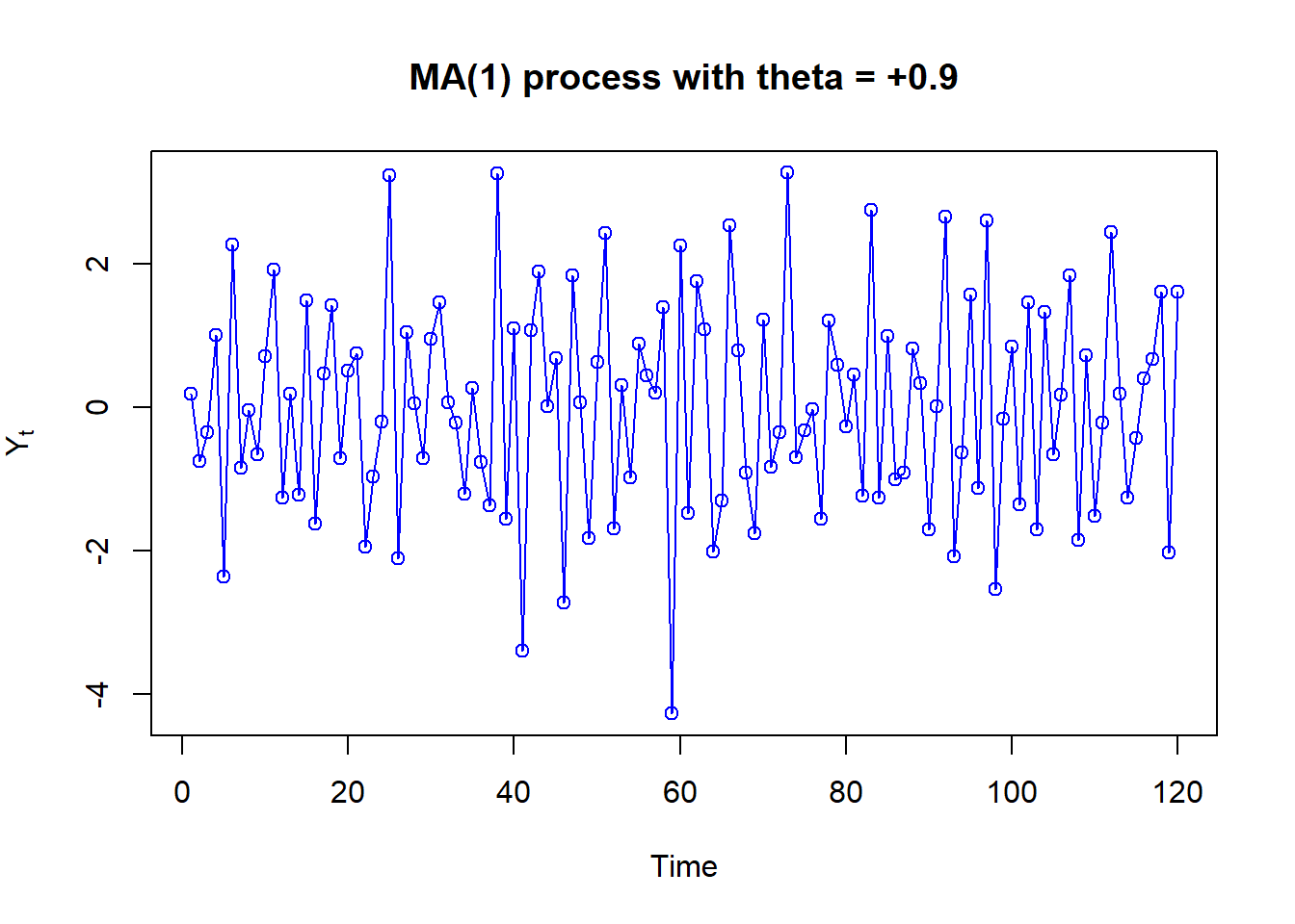

Code

par(mfrow = c(1, 2), mar = c(4, 4, 2, 2), oma = c(0, 0, 2, 0))
# Lag plot Yt vs Y_(t-1) for MA(1) th=+0.9
# with the lowess smoother
plot_lag_lowess(ma1.1.s, num_lags = 4)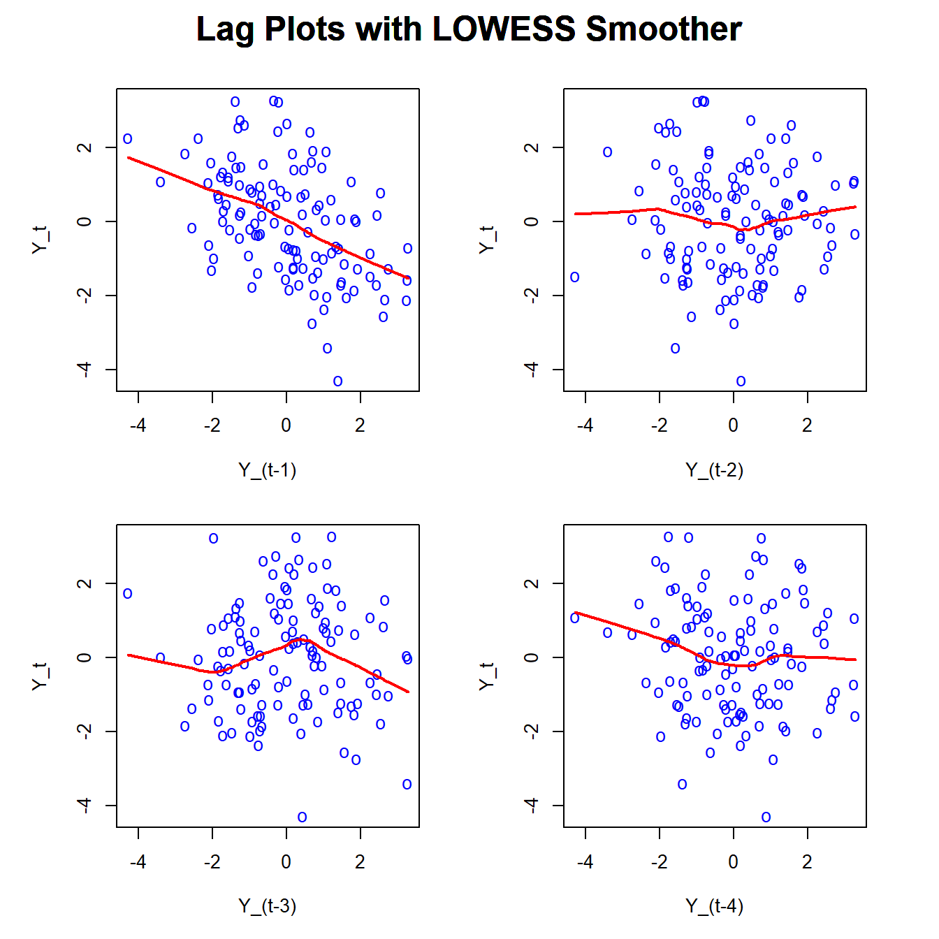

Code

# Time Plot of an MA(2) Process with theta1 = 1 and theta2 = -0.6
data(ma2.s)
plot(ma2.s,
     ylab=expression(Y[t]),
     type='o',
     xlab='Time',
     main='MA(2) process with theta1 = 1 and theta2 = -0.6',
     col = 'blue')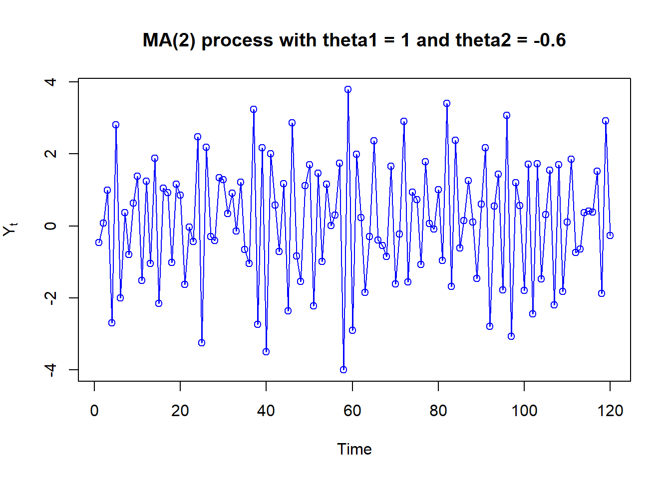

Code

par(mfrow = c(2, 2), mar = c(4, 4, 2, 2), oma = c(0, 0, 5, 0))

plot_lag_lowess(ma2.s, num_lags = 4)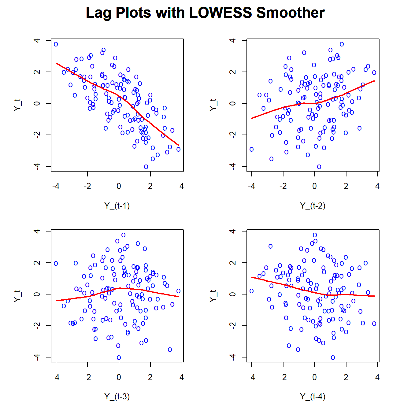

Code

# Auto-correlation function for several MA(1) and MA(2) models
par(mfrow = c(2, 2), mar = c(4, 4, 2, 2), oma = c(0, 0, 5, 0))

# Function to compute theoretical ACF for MA(1) process
compute_acf_ma1 <- function(theta, max_lag = 12) {
  acf_values <- numeric(max_lag + 1)
  acf_values[1] <- 1  # ACF at lag 0 is always 1
  acf_values[2] <- -theta / (1 + theta^2)

 for (k in 3:(max_lag + 1)) {
    acf_values[k] <- 0
  }
  return(acf_values)  # Include lag 0
}

# Function to plot ACF
plot_acf_ma1 <- function(theta, max_lag = 12) {
  lags <- 0:max_lag
  acf_values <- compute_acf_ma1(theta, max_lag)

  plot(lags, acf_values, type = "h", lwd = 2, ylim = c(-1, 1),
       xlab = "Lag", ylab = expression(rho[k]), main = "", axes = FALSE)
  points(lags, acf_values, pch = 19, cex = 1.5)

  axis(1, at = lags)
  axis(2, las = 1)
  abline(h = 0)

  text(max(lags) * 0.7, 
     max(abs(acf_values), na.rm = TRUE) * 0.8, 
     labels = bquote(theta == .(theta)), 
     cex = 1.2)

   # Label zero ACF values
  zero_lags <- which(acf_values == 0)
  text(lags[zero_lags], 
       acf_values[zero_lags], 
       labels = "0", 
       pos = 3, 
       cex = 0.8)
}

compute_acf_ma2 <- function(theta1, theta2, max_lag = 12) {
  acf_values <- numeric(max_lag + 1)
  acf_values[1] <- 1  # ACF at lag 0 is always 1

  acf_values[2] <- -theta1 / (1 + theta1^2 + theta2^2)
  acf_values[3] <- -theta1 * theta2 / (1 + theta1^2 + theta2^2)

  for (k in 4:(max_lag + 1)) {
    acf_values[k] <- 0
  }
  return(acf_values)  # Include lag 0
}

plot_acf_ma2 <- function(theta1, theta2, max_lag = 12) {
  lags <- 0:max_lag
  acf_values <- compute_acf_ma2(theta1, theta2, max_lag)

  plot(lags, acf_values, type = "h", lwd = 2, ylim = c(-1, 1),
       xlab = "Lag", ylab = expression(rho[k]), main = "", axes = FALSE)
  points(lags, acf_values, pch = 19)

  axis(1, at = lags)
  axis(2, las = 1)
  abline(h = 0)

  label_text <- bquote(theta[1] == .(theta1) ~ "," ~ theta[2] == .(theta2))

  text(max(lags) * 0.7, 
      max(abs(acf_values), na.rm = TRUE) * 0.8, 
      labels = label_text, 
      cex = 1.2)
  # Label zero ACF values
  zero_lags <- which(acf_values == 0)
  text(lags[zero_lags], 
       acf_values[zero_lags], 
       labels = "0", 
       pos = 3, 
       cex = 0.8)
}

# Plot for different theta values
plot_acf_ma1(0.9)
plot_acf_ma1(-0.9)
plot_acf_ma2(0.5, 0.25)
plot_acf_ma2(1.0, -0.25)
# Main title
mtext("Theoretical ACFs for various MA(1) and MA(2)", 
      outer = TRUE, 
      cex = 1.8, 
      line = 2, 
      font = 2)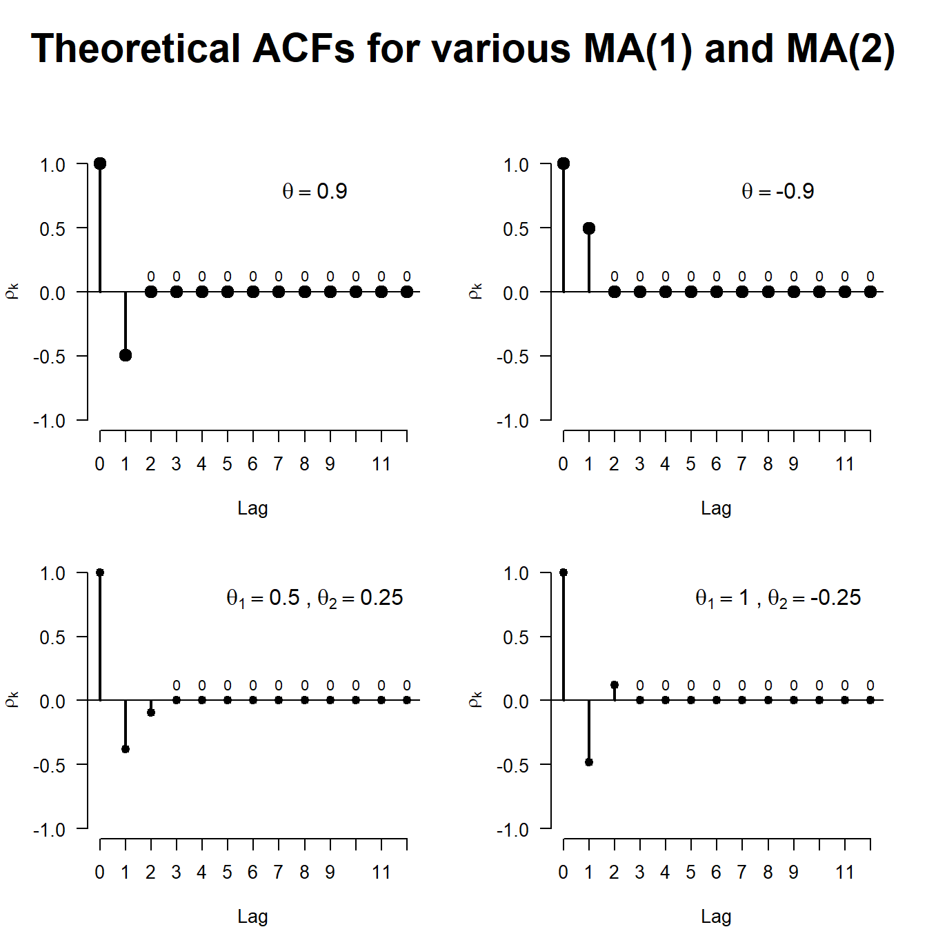

1.2 AR(p) processes

Code

# Auto-correlation function for several AR(1) models
par(mfrow = c(2, 2), mar = c(4, 4, 2, 2), oma = c(0, 0, 5, 0))

# Function to plot theoretical ACF for AR(1) process
plot_acf_ar1 <- function(phi, max_lag = 12) {
  lags <- 0:max_lag
  acf_values <- phi^lags
  
  plot(lags, acf_values, type = "h", lwd = 2, ylim = c(-1, 1),
       xlab = "Lag", ylab = expression(rho[k]), main = "", axes = FALSE)
  points(lags, acf_values, pch = 19, cex = 1.5)
  
  axis(1, at = lags)
  axis(2, las = 1)
  abline(h = 0)
  
  text(max_lag * 0.7, 
      max(acf_values) * 0.8, 
      labels = bquote(phi == .(phi)), 
      cex = 1.2)
  # Label zero ACF values
  zero_lags <- which(acf_values == 0)
  if (length(zero_lags) > 0)
  {
  text(lags[zero_lags], 
       acf_values[zero_lags], 
       labels = "0", 
       pos = 3, 
       cex = 0.8)
  }
}

# Plot for different phi values
plot_acf_ar1(0.9)
plot_acf_ar1(0.4)
plot_acf_ar1(-0.8)
plot_acf_ar1(-0.5)
# Main title
mtext("Theoretical ACFs for various AR(1) Models", 
      outer = TRUE, 
      cex = 1.8, 
      line = 2, 
      font = 2)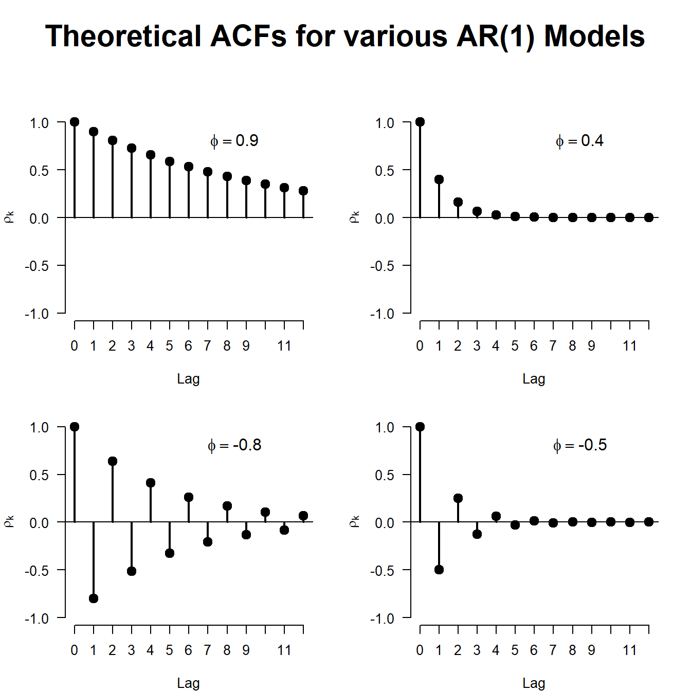

Code

# Time plot of an AR(1) process with phi = 0.9
data(ar1.s)
plot(ar1.s,
     ylab=expression(Y[t]),
     type='o',
     xlab='Time',
     main='AR(1) process with phi = 0.9',
     col = 'blue')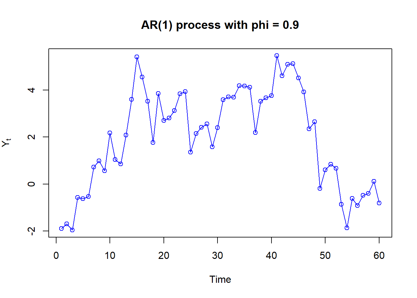

Code

# Lag plots Yt vs Y_(t-k) for an AR(1) process with phi = 0.9
plot_lag_lowess(ar1.s, num_lags = 4)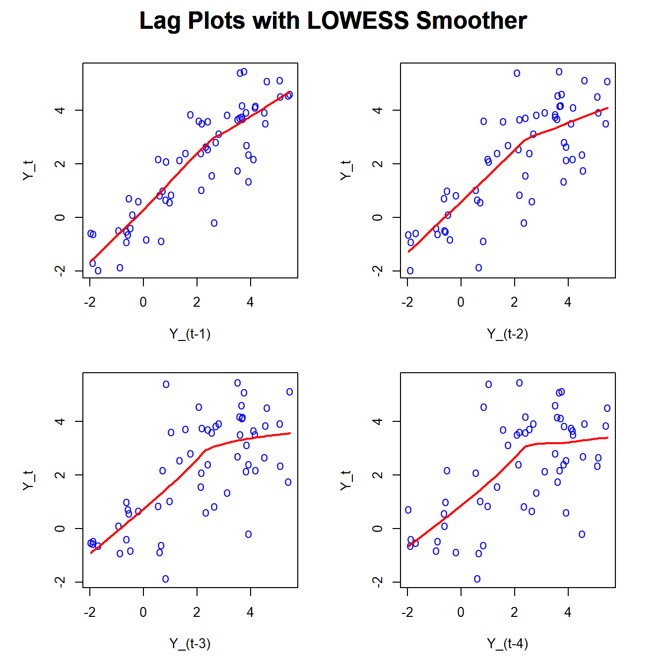

Code

# Auto-correlation function for several AR(2) models
par(mfrow = c(2, 2), mar = c(4, 4, 2, 2), oma = c(0, 0, 5, 0))

# Function to compute theoretical ACF for AR(2) process
compute_acf_ar2 <- function(phi1, phi2, max_lag = 12) {
  acf_values <- numeric(max_lag + 1)
  acf_values[1] <- 1  # ACF at lag 0 is always 1

  # Solve Yule-Walker equations for first two autocorrelations
  acf_values[2] <- phi1 / (1 - phi2)
  acf_values[3] <- (phi2*(1-phi2) + phi1^2) / (1 - phi2)

  # Recursively compute the rest
  for (k in 4:(max_lag + 1)) {
    acf_values[k] <- phi1 * acf_values[k - 1] + phi2 * acf_values[k - 2]
  }

  return(acf_values)  # Include lag 0
}

# Function to plot ACF
plot_acf_ar2 <- function(phi1, phi2, max_lag = 12) {
  lags <- 0:max_lag
  acf_values <- compute_acf_ar2(phi1, phi2, max_lag)

  plot(lags, acf_values, type = "h", lwd = 2, ylim = c(-1, 1),
       xlab = "Lag", ylab = expression(rho[k]), main = "", axes = FALSE)
  points(lags, acf_values, pch = 19)

  axis(1, at = lags)
  axis(2, las = 1)
  abline(h = 0)

  label_text <- bquote(phi[1] == .(phi1) ~ "," ~ phi[2] == .(phi2))

  text(max(lags) * 0.7, 
      max(acf_values, na.rm = TRUE) * 0.8, 
      labels = label_text, 
      cex = 1.2)
  # Label zero ACF values
  zero_lags <- which(acf_values == 0)
  if (length(zero_lags) > 0)
  {
  text(lags[zero_lags], 
       acf_values[zero_lags], 
       labels = "0", 
       pos = 3, 
       cex = 0.8)
  }
}

# Plot for different phi1 and phi2 values
plot_acf_ar2(0.5, 0.25)
plot_acf_ar2(1.0, -0.25)
plot_acf_ar2(1.5, -0.75)
plot_acf_ar2(1.0, -0.6)
# Main title
mtext("Theoretical ACFs for various AR(2) Models", 
      outer = TRUE, 
      cex = 1.8, 
      line = 2, 
      font = 2)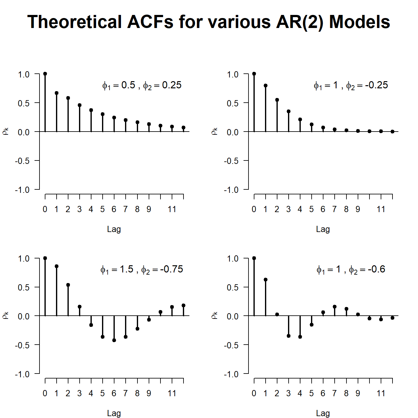

Code

# Time plot of an AR(2) process with phi1 = 1.5 and phi2 = -0.75
data(ar2.s)
plot(ar2.s,
     ylab=expression(Y[t]),
     type='o',
     xlab='Time',
     main='AR(2) process with phi1 = 1.5 and phi2 = -0.75',
     col = 'blue', 
     xaxt = 'n')
axis(1, at = seq(0, length(ar2.s), by = 12))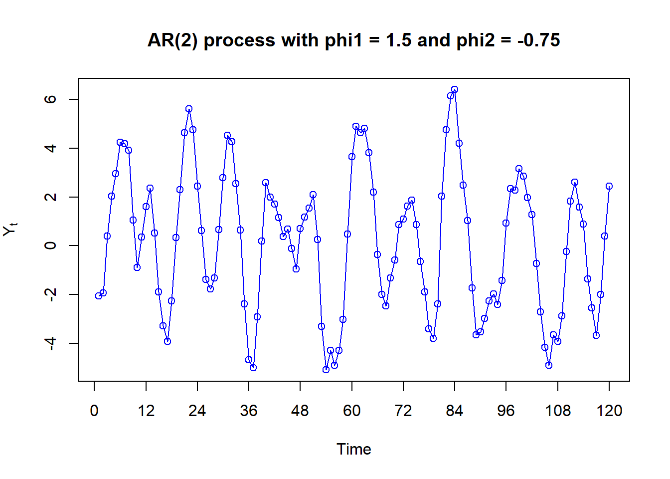

1.3 ARMA(p,q) processes

Code

# ARMA(1,1) process
data(arma11.s)
plot(arma11.s,
     ylab=expression(Y[t]),
     type='o',
     xlab='Time',
     main='ARMA(1,1) process with phi = 0.6 and theta = -0.3',
     col = 'blue')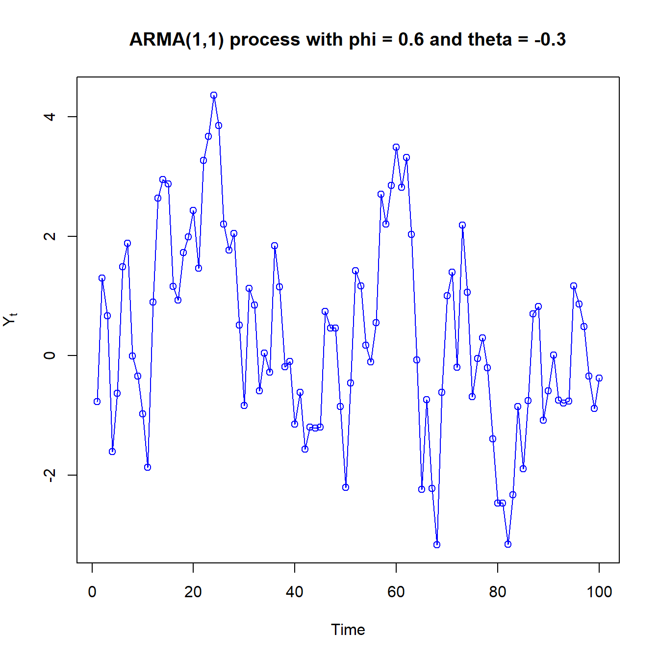

Code

# Lag plots Yt vs Y_(t-k) for an ARMA(1,1) process with phi = 0.6 and theta = -0.3

plot_lag_lowess(arma11.s, num_lags = 4)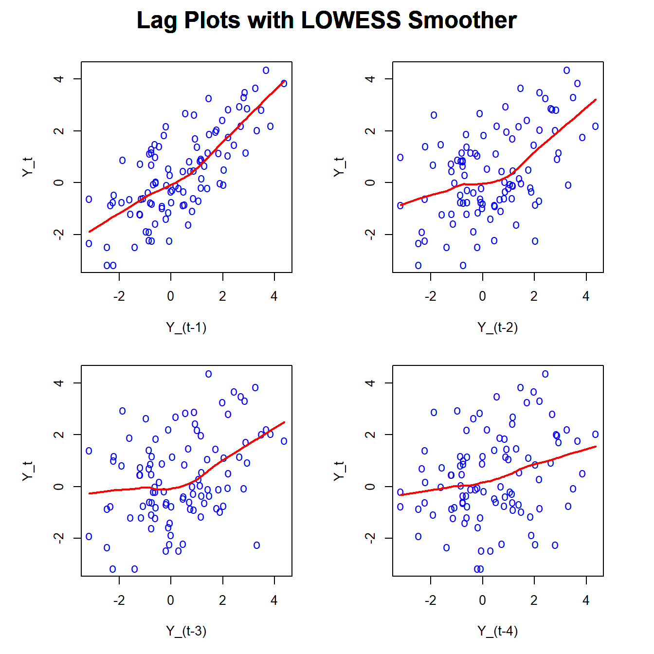

Code

# Auto-correlation function for ARMA(1,1) model
par(mfrow = c(2, 2), mar = c(4, 4, 2, 2), oma = c(0, 0, 5, 0))

# Function to compute theoretical ACF for ARMA(1,1) process
compute_acf_arma11 <- function(phi, theta, max_lag = 12) {
  acf_values <- numeric(max_lag + 1)
  acf_values[1] <- 1  # ACF at lag 0 is always 1


  # Recursively compute the rest
  for (k in 2:(max_lag + 1)) {
    acf_values[k] <- (1-theta*phi)*(phi-theta)*phi^(k-1)/(1-2*theta*phi+theta^2)
  }

  return(acf_values)  # Include lag 0
}

# Function to plot ACF
plot_acf_arma11 <- function(phi, theta, max_lag = 12) {
  lags <- 0:max_lag
  acf_values <- compute_acf_arma11(phi, theta, max_lag)

  plot(lags, acf_values, type = "h", lwd = 2, ylim = c(-1, 1),
       xlab = "Lag", ylab = expression(rho[k]), main = "", axes = FALSE)
  points(lags, acf_values, pch = 19)

  axis(1, at = lags)
  axis(2, las = 1)
  abline(h = 0)

  label_text <- bquote(phi == .(phi) ~ "," ~ theta == .(theta))

  text(max(lags) * 0.7, 
      max(acf_values, na.rm = TRUE) * 0.8, 
      labels = label_text, 
      cex = 1.2)

  # Label zero ACF values
  zero_lags <- which(acf_values == 0)
  if (length(zero_lags) > 0)
  {
  text(lags[zero_lags], 
       acf_values[zero_lags], 
       labels = "0", 
       pos = 3, 
       cex = 0.8)
  }
}

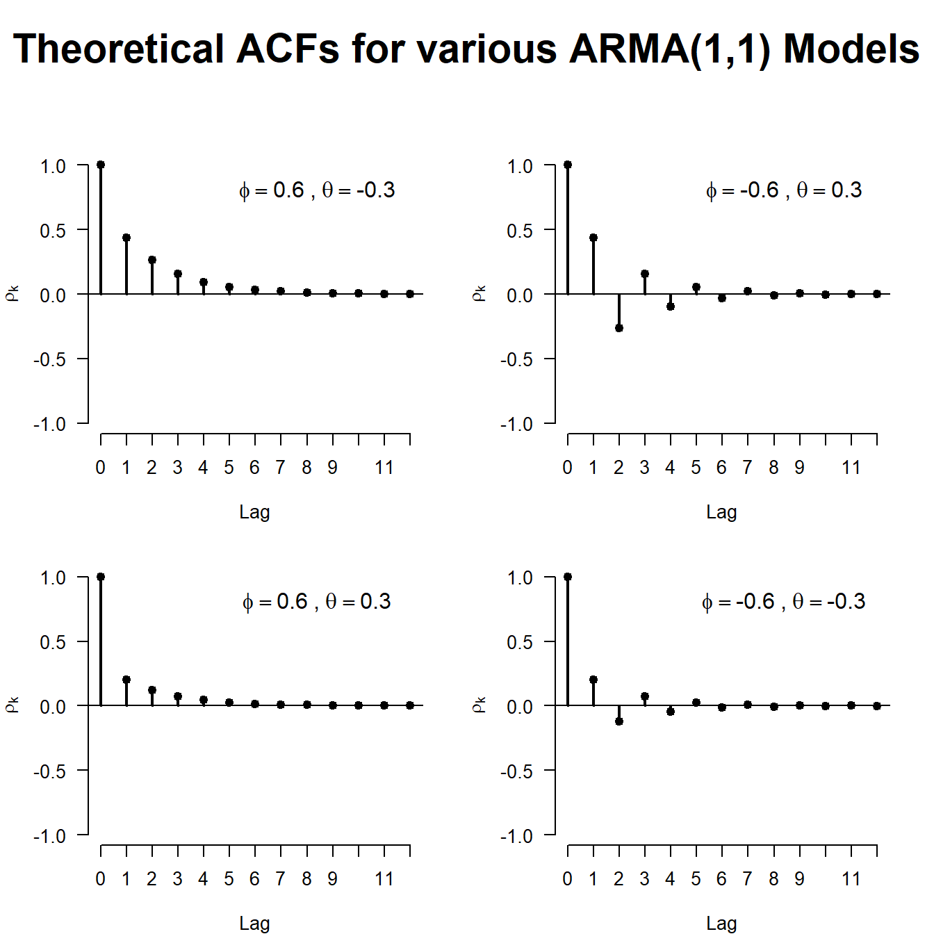
# Plot for different phi and theta values
plot_acf_arma11(0.6, -0.3)
plot_acf_arma11(-0.6, 0.3)
plot_acf_arma11(0.6, 0.3)
plot_acf_arma11(-0.6, -0.3)
# Main title
mtext("Theoretical ACFs for various ARMA(1,1) Models", 
      outer = TRUE, 
      cex = 1.8, 
      line = 2, 
      font = 2)